Introduction
Welcome to this breakdown of our texture creation process.
In this guide we will be going over our workflow for creating a fully tileable photoscanned surface. While we won’t be covering any single topic in great detail, our aim is to provide a comprehensive document that can be used as a guide by anyone who wants to create their own photogrammetry-based textures.
What is a “photoscanned” texture?
Photogrammetry or photoscanning refers to the process of taking multiple overlapping photos of an object or surface, and then using special photogrammetry software like Reality Capture to create a highly accurate 3d version of it by cross-referencing points in different photos and using maths to figure out where everything sits in 3d space.
How are photoscanned textures different from other kinds of textures?
Since photogrammetry is capable of building such accurate 3d versions of real surfaces, this generally makes it much more realistic than other methods like manual painting, procedural generation, or estimating displacement/normal information based on any single input texture. Once we have a scan of a surface, it becomes a simple matter to extract all the necessary real-world information from it like displacement, normal, color, ambient-occlusion, etc.
Step 1: Photography

There are already many resources available that demonstrate different techniques to photoscanning surfaces for the purpose of texture creation, so rather than describe it in detail here, we simply recommend these videos:
- Photogrammetry workflow for surface scanning with the monopod – Gravel PBR Material
- Outdoor Photogrammetry Surface Scanning for Materials with a Flash
- https://80.lv/articles/photogrammetry-almanac-environment-pbr-texture-creation
In a nutshell, you want to capture around 300 images per 2 metre square area, with as equal spacing between shots as possible.
Shooting with a cross-polarized flash setup is ideal for all surfaces to avoid reflections and overpower the natural lighting, but for rough surfaces you can sometimes get away with simply shooting on an overcast day or in a shaded area, and rely on delighting techniques later on.
It helps to place a pair of measuring tapes on each axis of the area you want to scan, which serves both as a spacing aid while shooting, and a reference later on for calibrating the scale of the final material.
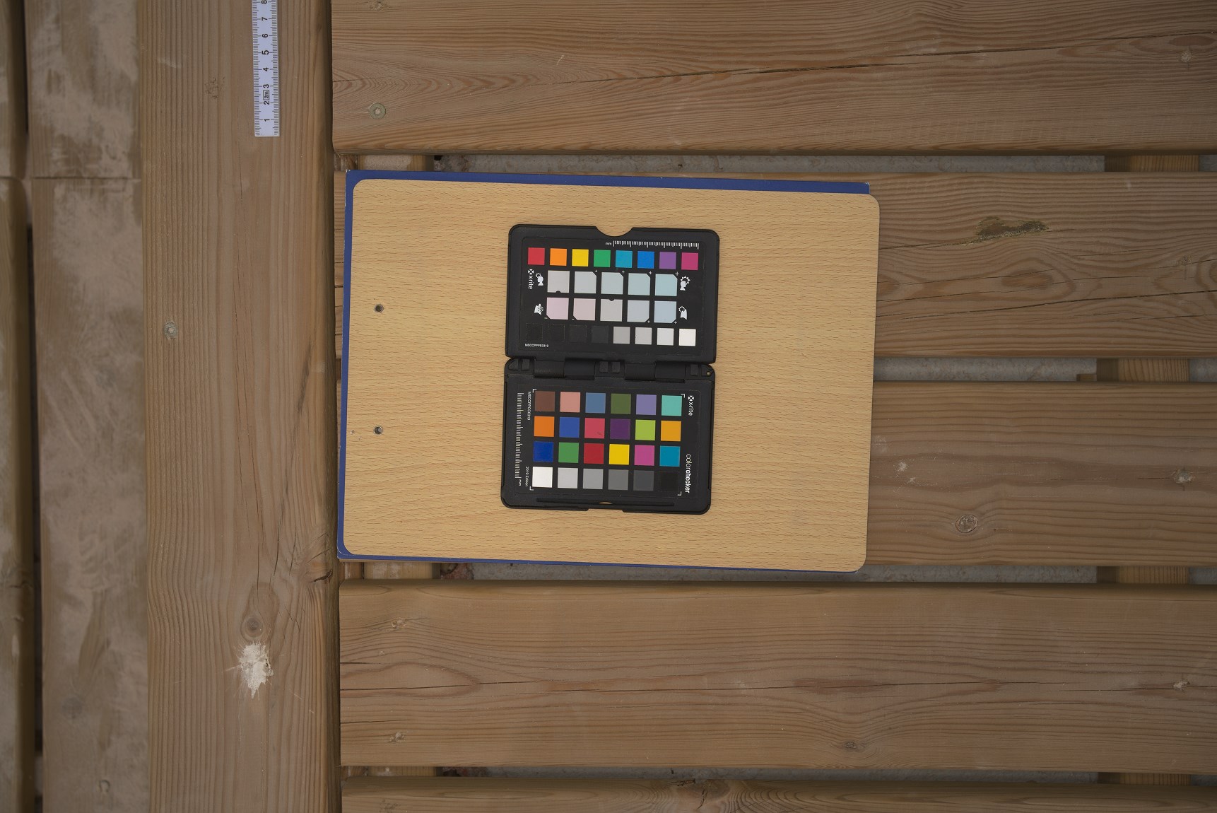
It’s also important to include a color chart in the scan area – preferably just outside, but definitely on the same plane as the surface you are scanning.
Finally, we recommend shooting a number of additional reference/contextual photos, especially one that highlights the specular properties of your surface, to help you build an accurate material later on.
Step 2: Adjust/sort input photos in RawTherapee or Darktable
Before starting any new scan project, we need to process our raw photos in a free application like RawTherapee or Darktable. We do not recommend Adobe Lightroom is it’s difficult to make photos linear which is important for color accuracy.
While most photogrammetry software can import raw files directly, we want to do certain batch processes on all the photos simultaneously before exporting them, like brightness adjustments, white-balance fixes, vignette removal, and chromatic aberration removal.
Keep in mind we don’t want to do any adjustments that will confuse the photogrammetry software. Generally, this means we have to stay away from filters like sharpen, denoise, and so on, since those will treat individual pixel clusters differently on each photo, and we ideally need to stick to filters and adjustments that change all pixels universally across all the images (so things like brightness, contrast, and color balance are fine, vignette removal can be a little more tricky but usually also fine). After doing these adjustments we will export the Raws as 16-bit TIFF files.
Note: It is highly recommended to export 16-bit files like TIFF. They are incredibly large and will take up a lot of space on your hard drive, but you can delete them after you are done with the project, since you will still have your Raws. While you can use other formats, we have found that things like PNG are far too slow to load/save, and formats like EXR, while small and fast, will create problems when exporting the texture bakes from Reality Capture later in the process. Never export your photos in 8bit regardless of format, as this will effectively prevent you from doing any color adjustments to your textures later on, which is handy for making the roughness map.
The RawTherapee process:
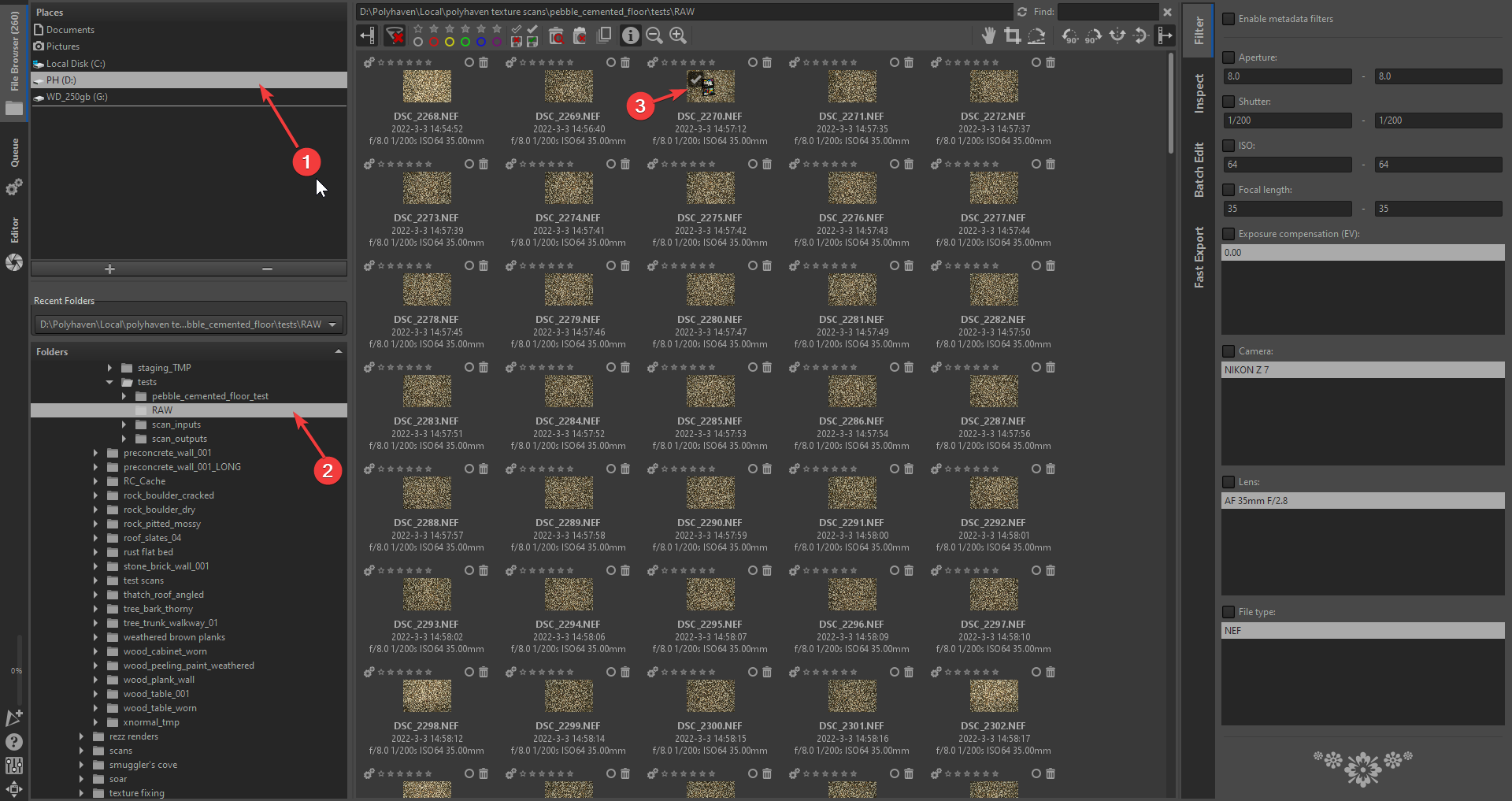
- To import a new batch of photos to RawTherapee, click the File Browser tab at the top left of the UI, and navigate to the folder containing all your photos. It’s a good idea to start with the color-balance adjustments, so double-click on your color chart shot to open it up.
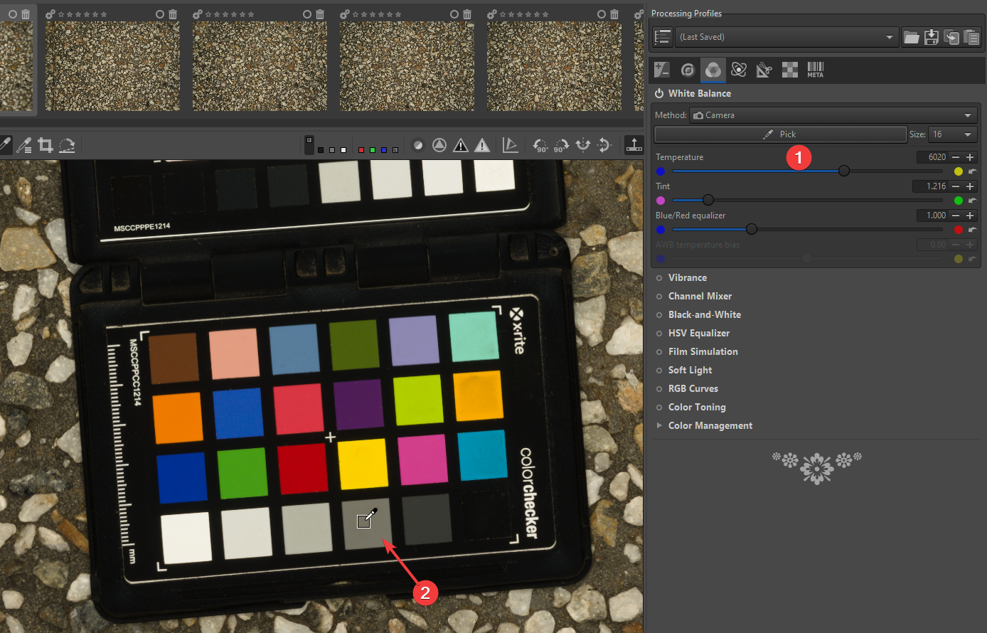
- With the color chart opened, we can set the white balance by clicking on the “Color” tab on the right, (shortcut: ALT+C) and use the white-balance picker to sample one of the grey tones on the bottom of the color chart. The software will use this grey information to automatically figure out an accurate, “neutral” white balance.
Note: We describe our color calibration process in more detail here. This process is important if you want to make accurate PBR materials that work in any lighting conditions.
- Once we have the white balance, we can right click on the image thumbnail at the top of the window, and go to Processing Profile Operations > Copy to copy the white balance information we just created, and paste it onto all the other images by SHIFT-selecting them all, right clicking, and selecting Processing Profile Operations > Paste
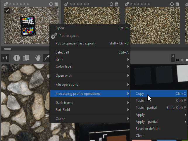

NOTE: Most operations can be copied to all the other images using the CTRL+C/CTRL+V shortcuts in this manner. Or we can paste partial operations using CTRL+SHIFT+V.
- Each batch of photos will need different treatment. For example some batches will need brightness and contrast adjustments (found in the exposure tab, shortcut: ALT+E) or we may need to crop certain images that have undesired elements by going to the Transform tab (Shortcut: ALT+T).
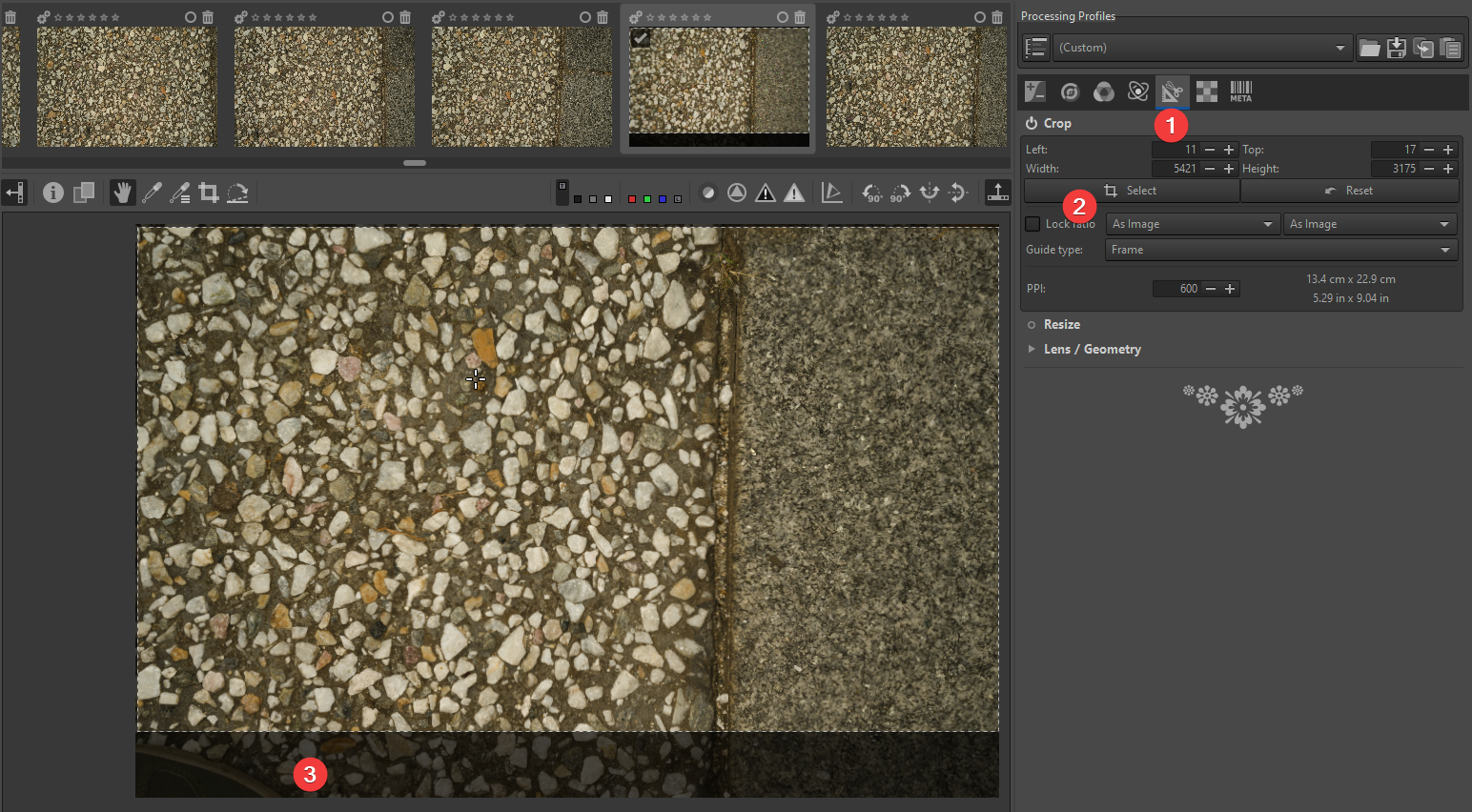
NOTE: Crop operations can also be copied to multiple images. This is especially useful for cropping out shoes or tripod-legs if they appear in multiple photos, since these will most likely be in more or less the same areas of the image. As a rule, it’s usually better to crop out undesired elements (if possible) than to delete entire photos, since we need every bit of pixel information we can get in order to build a great scan.
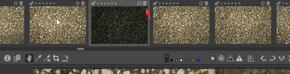
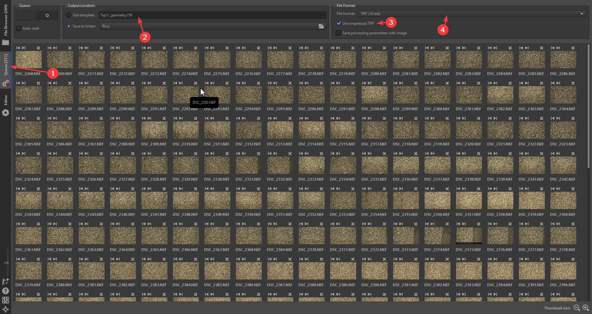
- Once we’ve done our adjustments and cropped out any undesired elements, we should go through the entire batch of photos and delete any blurry or noisy images that we see. This can be very time consuming on large datasets, and it’s sometimes not feasible to look at every single image in detail. Still, it’s a good idea to at least just scroll through briefly and investigate any photos that look a bit weird, even if we’re just looking at thumbnails mostly:
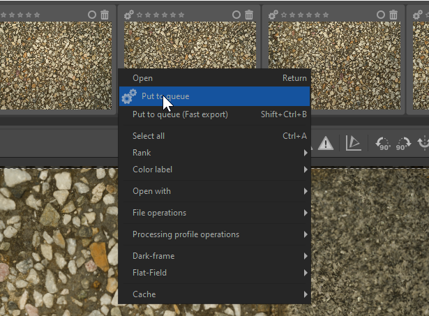
- Finally, we need to export our adjusted photos. To do this, we shift-select all the images we want to export and right click, selecting Put to Queue:
Then we select the queue tab on the very left of the screen to view all the images. Here we can set our save location, export format and bit-depth. Again, it’s highly recommended to use something like uncompressed 16bit Tiff files:
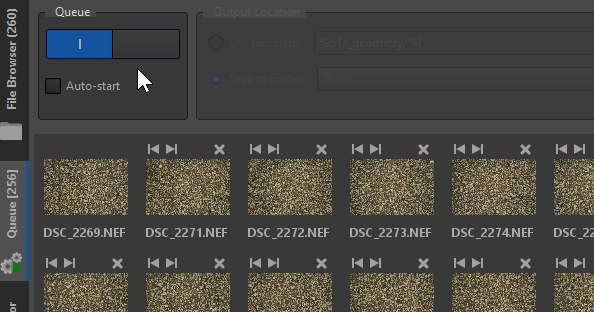
Now we can go ahead and click the Queue button, and wait a while for the batch to finish exporting:
RawTherapee Dos and Don’ts (summary):
Do:
- Set the correct white balance on the entire photo set, using the provided color chart. Like with many of the adjustments we do to photosets, this should be done as a batch process.
- Crop out any anomalies on individual photos, of things that we don’t want in the scan. This especially includes anything that moves, (e.g. leaves, rocks or grass that obviously moved during the shoot). Scanning software will be confused by moving objects, since it needs static shapes to cross reference between images in order to build a reliable point cloud.
- If necessary set the exposure/contrast. Usually it’s best to keep this subtle, and do it as a batch process as well if we can. Normally if the light changes during a shoot (as it often does), it can be ignored unless it’s a really harsh shift. It seems Reality Capture is generally better at recognizing shapes and not relying too much on value information.
- Reduce any vignette effects. (Heavy vignetting is sometimes a result of using a polarised flash setup in a dimly lit environment.) It’s best to remove the vignette since if we leave it in the resulting texture may be slightly darker than it should be.
Do Not:
- Any kind of cloning, painting or general process that alters photos on a per-pixel level. This also mostly includes things like noise removal and sharpening filters. It may still be possible to do those things in limited cases, but altering individual photos in this way will result in issues in the build step. It’s often better to just delete a blurred photo entirely, than trying to rescue it.
Step 3: RealityCapture processing
The next step is to load our images into our photogrammetry software of choice. We use Reality Capture which is most often recommended for photoscanning in general, however note that it is paid software that charges per input. It is particularly good for surface texture scanning. Other alternatives are 3DF Zephyr and Metashape, which are also commonly used for this purpose.
A typical scan of 300 images with a 24MP camera will cost around $5. The more images you shoot and the higher resolution your camera, the more expensive the scan and the more intense the hardware requirements, however this also results in higher quality outputs.
Once the inputs are paid for in Reality Capture, you’re free to re-process the scan and export any data as much as you like. You also only pay at the end when you’re ready to export, leaving you free to play around and experiment before needing to make any purchases.
Meshroom is a decent free alternative, but we generally don’t recommend it because it’s slow and requires a lot of fiddling to get decent results.
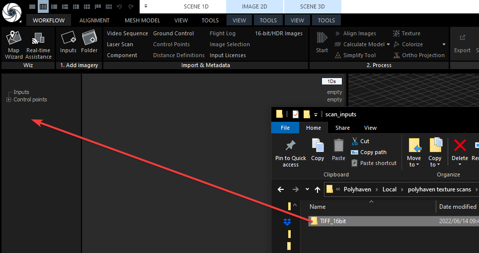
- Simply drag the entire folder of your exported TIFFs into RealityCapture.
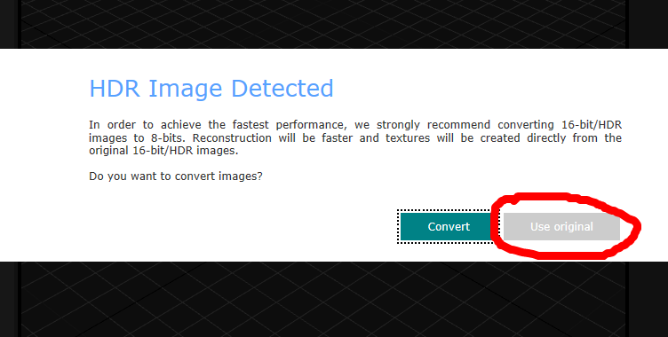
Reality Capture will give us a little popup asking whether we’d like to convert the images to 8bit on import, or whether we want to use the original 16bit ones. While RC highly recommends using the converted 8-bit images, in our tests this actually does nothing to improve performance and just wastes time converting and dealing with multiple image sets. Rather click “Use original”:
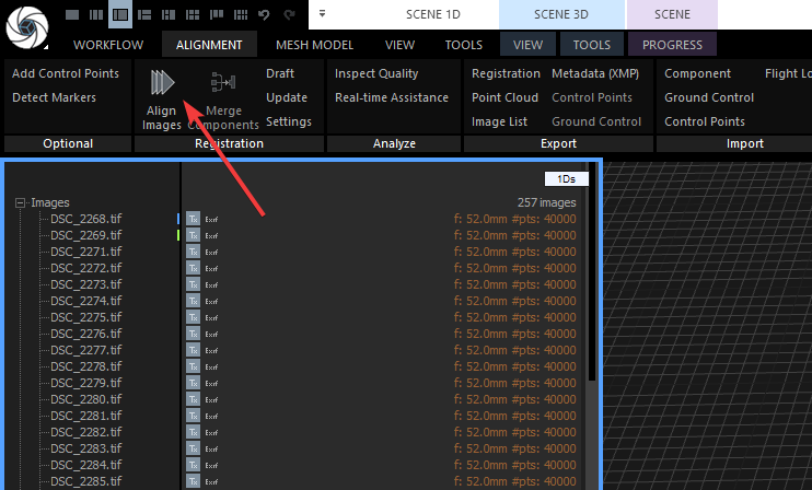
Once we have the images imported, we can go to the alignment tab at the top of the screen and click “Align Images”. This can take a few minutes, depending on the amount and resolution of the images.
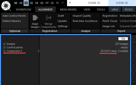
- After the images have been aligned, we can check the component item in the 1Ds view on the left to see how many photos were aligned. There’s no reason for concern if it misses a few. The more the better of course.
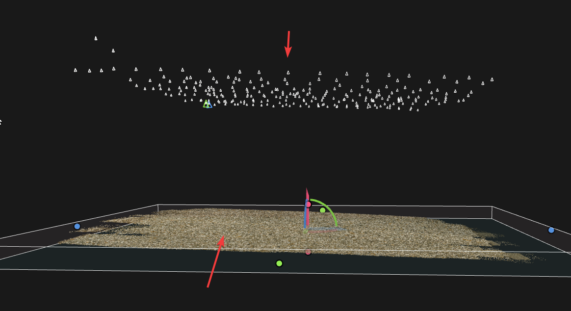
We can also check the pointcloud in the 3Ds view to get an idea of how accurate the build was. Here we can see the cameras (at the top) look pretty consistent, and the point cloud at the bottom looks flat and consistent as expected. We can also drag/rotate the bounding box in the 3d view to crop the scan down to the area we want. (Cropping down the scan will save time during the next steps) Use the colored dots to scale the bounding box, and use the widget in the center to rotate and move it.
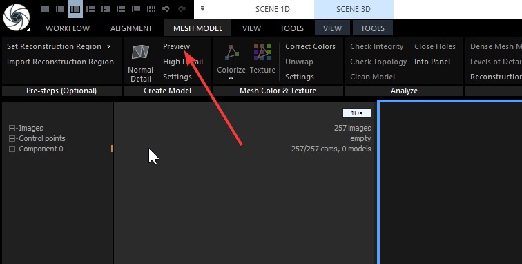
Optional: If necessary we can also build a low-detail preview version of the scan to get an even clearer idea of what it will look like:
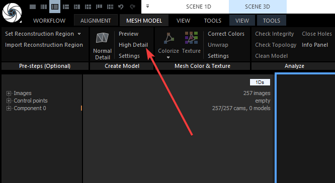
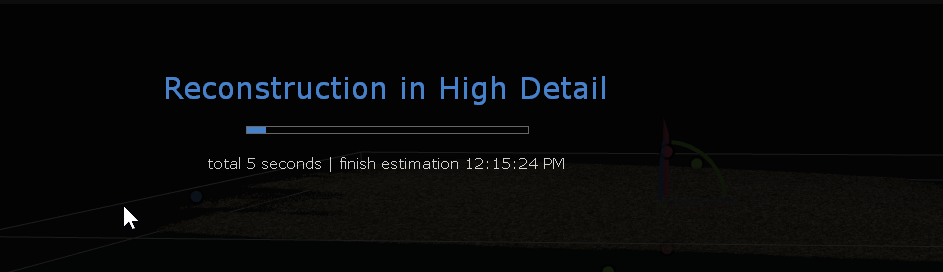
- Once we’re happy with the pointcloud we can go ahead and build the high-detail scan. This can take a lot of time (several hours) depending on the speed of the PC we’re working on, and the amount/resolution of input photos provided. It is now building a super dense mesh with potentially hundreds of millions of triangles.
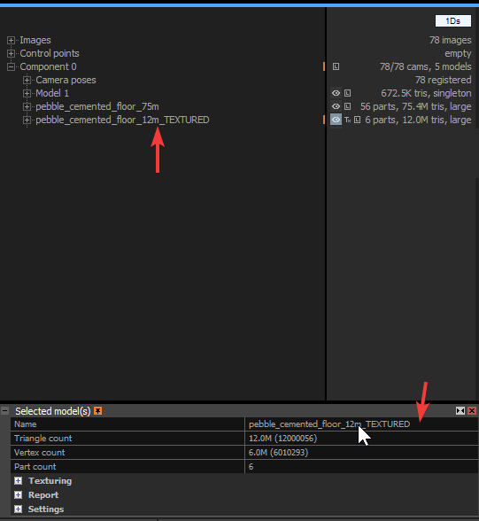
When it’s done, we can click on the generated mesh in the 1Ds view and give it a name. It’s a good idea to keep everything organized, since we’re going to be creating 2 versions of the scan for baking as well as a third, low-detail proxy mesh which will be imported to Blender in order to align the bake-plane.
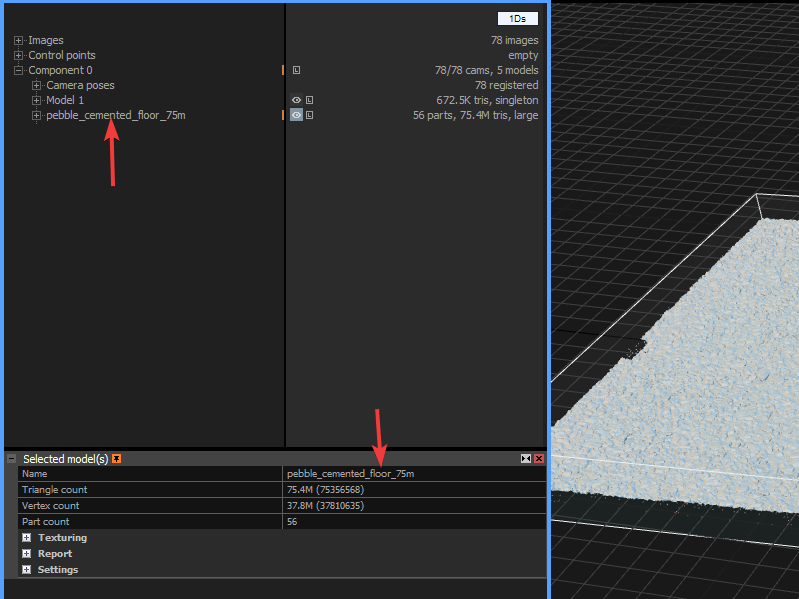
Here we’ve added “_75m” to the mesh name to indicate the triangle count for easy reference later on. We determine the triangle count by looking at the right-hand section in the 1Ds view.
Creating different meshes for baking: We will be using the initial high-detail mesh to bake the height and normal maps, but we’ll create a separate, lower detail version of the mesh for the color bake using RealityCapture’s simplify tools. (At 75m polygons the main mesh will be a pain to unwrap and texture-project, and it can also cause memory issues when baking)
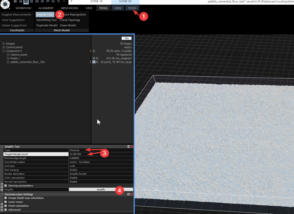
- Now we can create the simplified version of the mesh for texture projection. With the high-res mesh selected, go to Tools > Simplify Tool, and in the tool settings we can set the Type to Absolute, and the target triangle count to somewhere around 10-20 million (depending on the complexity of the original), and then click Simplify:
The simplify process will take a short while, when it’s done we can also select and rename it. We can also add “_TEXTURED” to the name, so that we don’t get confused later on when baking.
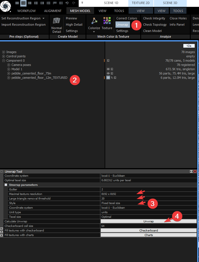
- Before we can project the color information onto this new mesh, we first need to unwrap it. With the _TEXTURED model selected, go to Mesh Model > Unwrap and under the Unwrap Parameters section change the resolution to what we want. In this case we’ll use 8192×8192, and we’ll set the large triangle removal threshold to 20. For the Style we can use Fixed texel size. Now go ahead and click Unwrap.
When it’s done we can expand the model in the 1Ds view, and because we selected Fixed Texel size, it has created as many UV maps as needed (in this case 4 UV maps) to ensure 100% quality when projecting the texture onto the scan.
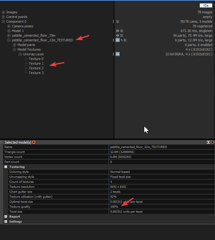
Note: Of course we will lose some quality when we bake the texture back down to a single plane, since it will be taking all the texture information from 4 UV maps and squeezing it all onto a single final map, but it’s usually best to project at the highest possible quality before baking regardless.
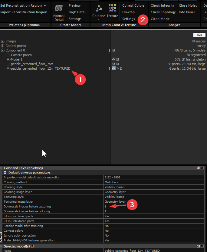
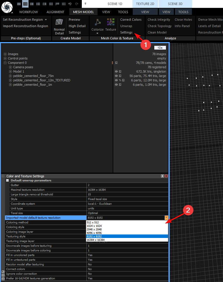
Now we need to set the texture downscale factor. To do this, click on the model and go to Mesh Model> Mesh Color & Texture > Settings and make sure Downscale Images Before Texturing is set to 1 to ensure maximum quality.
- Now, finally we can go ahead and project the texture. Select the _TEXTURED mesh and go to Mesh Model > Mesh Color & Texture and click Texture
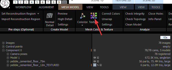
Note: Don’t use the Colorize button. This is for projecting vertex-colors onto the scan, and while useful in some cases (like really, really high-res geometry), it’s generally useless for getting sufficiently detailed color data on 8-16k surface scans.
The texture projection will take a while again, and when it’s done we should have the color information projected onto the scan like this:
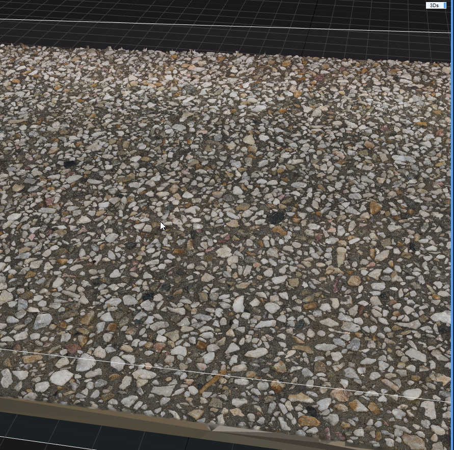
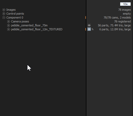
- Now we have the high-detail mesh ready for the Height/Normal bakes, and the lower-detail unwrapped/textured mesh which we’ll use for the color bake. This is what they look like in the outliner:
We need to export the scan to Blender so that we can align the bake plane to it. Exporting the high detail mesh will be very time consuming and Blender probably won’t even open it on most PCs. Therefore We can either export the 12m_TEXTURED mesh or we can create an even lower detail version. To do this we can just repeat the simplify step but make it something like 1-5 million triangles:

- We’ll select the mesh we want to export in the 1Ds view, go to Tools > Export > Mesh and PointCloud,
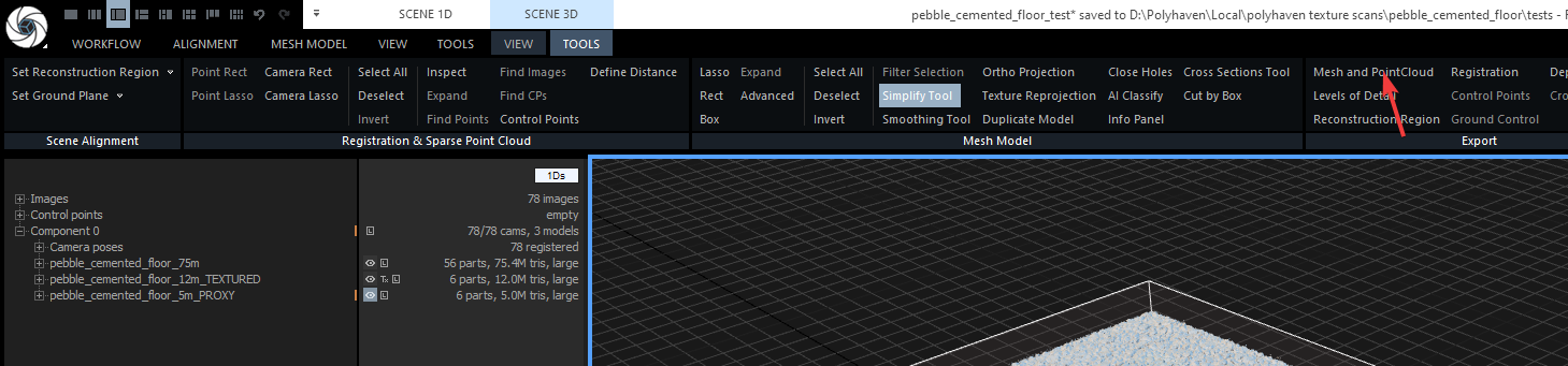
and in the export dialogue box set the location and filetype. In This case we’ll use OBJ as the filetype:
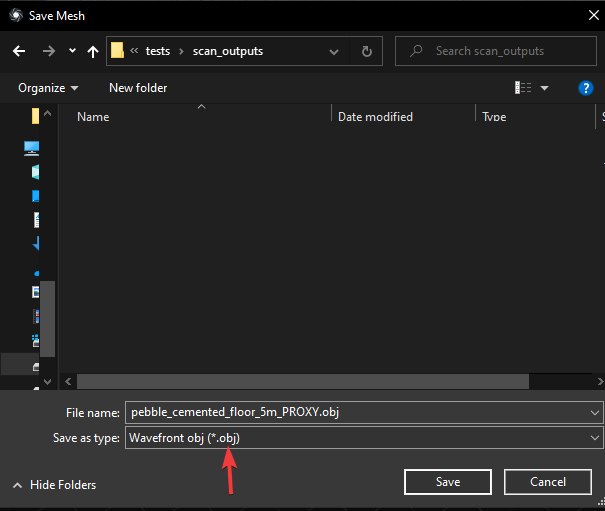
And click Save.
Note: At this point RealityCapture will ask us to pay up before we can export. We’ll select our payment method and save out the file.
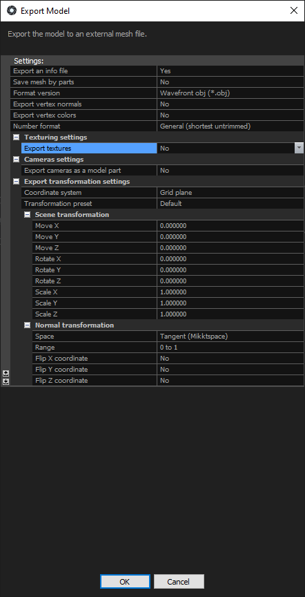
- Now we’ll get another dialog box to set a bunch of stuff before export. Use the settings shown in the screenshot below. These are important, since they will determine the orientation of our bake plane once we import it back in from Blender:
Step 4: Baking in RealityCapture
Overview
“Baking” is the process of transferring all the details of the scan onto individual texture maps (images), in order to make it easy for the end user to use these images and apply them to different objects and surfaces in a 3D scene.
There are many different types of maps, but usually when we bake we create only 3 important texture maps that all the other maps can be derived from. These 3 maps are the Color(also called “Diffuse” or “Albedo”), Displacement, and Normal maps.
Before we can bake the scan data onto texture maps, we first need to create a bake-plane in Blender. This plane will define the area of the scan that we want to transfer onto the texture maps.
Remember that the scan itself is in a very “messy” state. There are sometimes lots of glitches and artefacts on the edges and corners of the scan geometry, and we will want to avoid these as far as possible, so we’ll use the plane to find the best “clean” area on the scan.
Creating a bake-plane:
- In Blender, import the proxy version of the scan into Blender: File > Import > Wavefront(.obj)
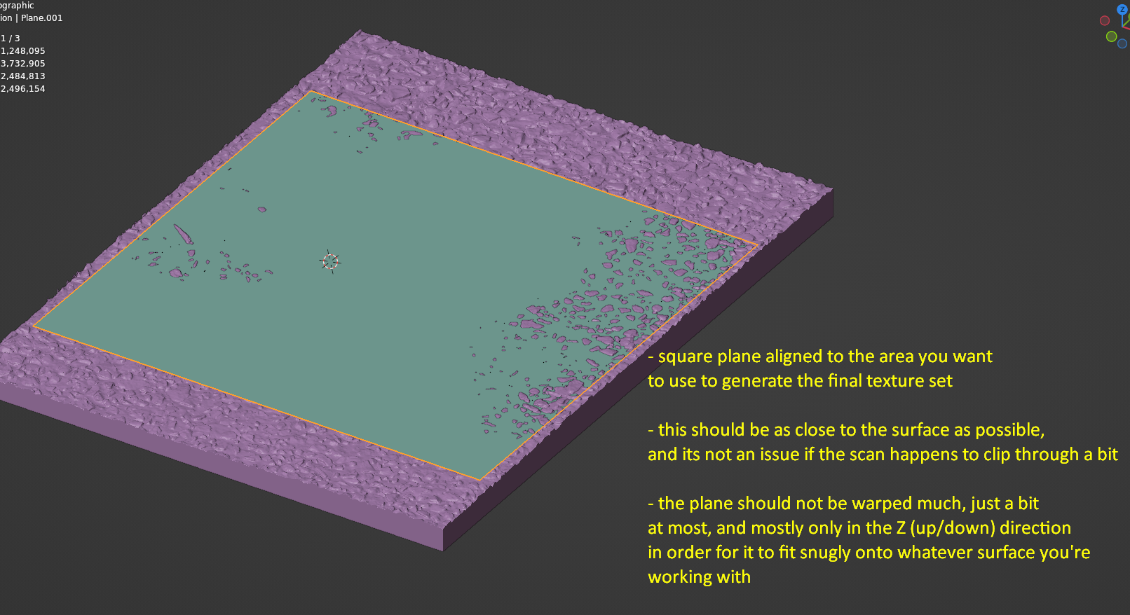
- We’ll use this proxy version of the scan to align the plane to the area we want to bake. It’s best to use the largest clean available area on the scan, and throughout the process we’ll try to keep the plane square, (i.e. don’t scale it on the X or Y axis). To add a plane, press SHIFT+A and click “Mesh > Plane”
- We’ll position the plane so that it hovers just above the scan. We’ll try to keep the plane an even distance above the average surface of the scan. It doesn’t matter if parts of the scan poke through the plane, as long as it’s hovering an average height of a few cm or mm above the surface.
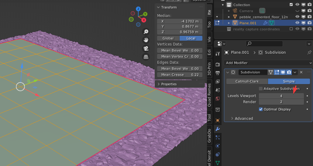
We can also add a few manual subdivisions to the plane (TAB into edit mode, select all verts and right-click > subdivide) and then slightly warp the plane using the proportional editing tool in order to make it fit the surface more snugly.

Note: If we do warp the plane, we just need to remember to add a subdivision modifier as well, (with about 3-4 levels) and to crease the outer edges using SHIFT+E. This is to make sure the plane remains really smooth, and no artefacts show up when baking. We should never warp the plane without using subdivisions to smooth it out afterwards, as this will almost certainly break the bake.
- Once the plane is positioned, we need to check that the normal direction is facing the correct way, and that the transformations are applied. To do this:
- Select the plane and press CTRL+A, then select “All Transforms” from the list. It’s important that the plane transforms are applied, even if the plane geometry itself is wherever/upside down etc.
- Make sure the plane Normals are facing “up” in relation to the scan surface, by clicking the “Viewport Overlays” button at the top of the 3d view, and then selecting “Face Orientation”. This will put a blue and red overlay over the objects in the scene. Blue means the Geometry Normals are all pointing the correct direction, Red means they are pointing the wrong direction:
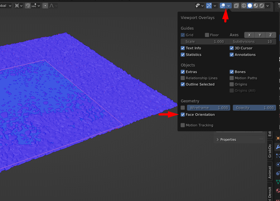
- Above we can see the plane normal direction is correct, since it shows up as blue.
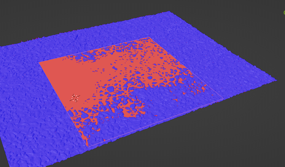
- Alternatively, if we have this situation in the above image where the plane shows up as red, we need to fix it by doing the following: Select the plane and press TAB to go into edit mode, then press A until all the vertices are selected, and finally press ALT+N to flip the normal direction. Now press TAB again to exit edit mode.
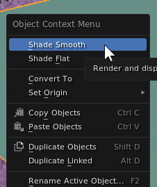
- We should also make sure the plane normals are set to smooth. To do this, select the plane, right-click and select Shade Smooth:
- When all the above is done, select the plane, hit File > Export > as obj, and make sure “Selection Only” is enabled at the top right:
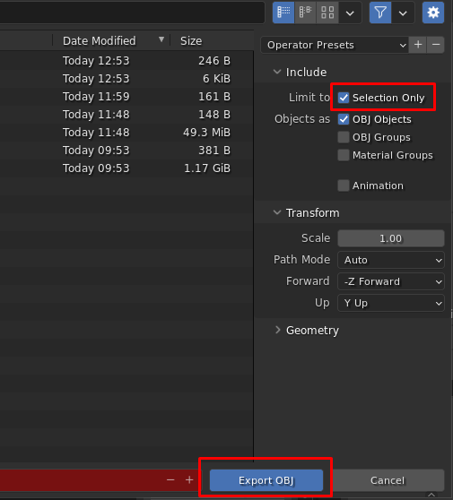
And click Export OBJ
Now we can start setting up the bake in RealityCapture:
- Before we import the bake plane, we need to set our default bake resolution. Go to Mesh Model > Settings and set the Imported-model default texture resolution. In this case we’ll use 8192×8192
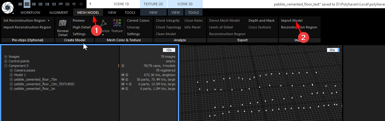
- Now we import the model by going to Mesh Model > Import Model
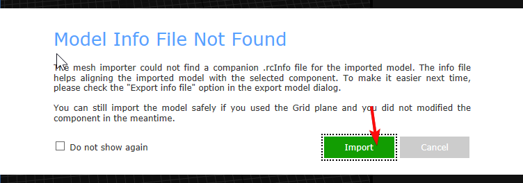
If we get a warning about Model Info Not Found, we just ignore it and click Import:
We should also rename our imported plane to something that makes sense like “Bake Plane”
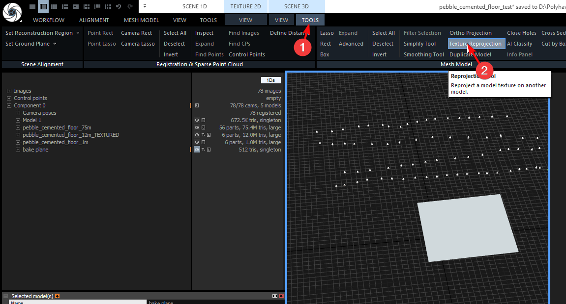
- When we are ready to bake, go to Tools > Texture reprojection
- We’ll bake the Normal and Displacement maps first, so in the Reprojection settings, set the source model to the highest detail geometry (in this case the 75m triangle version), and the result model to the bake plane:
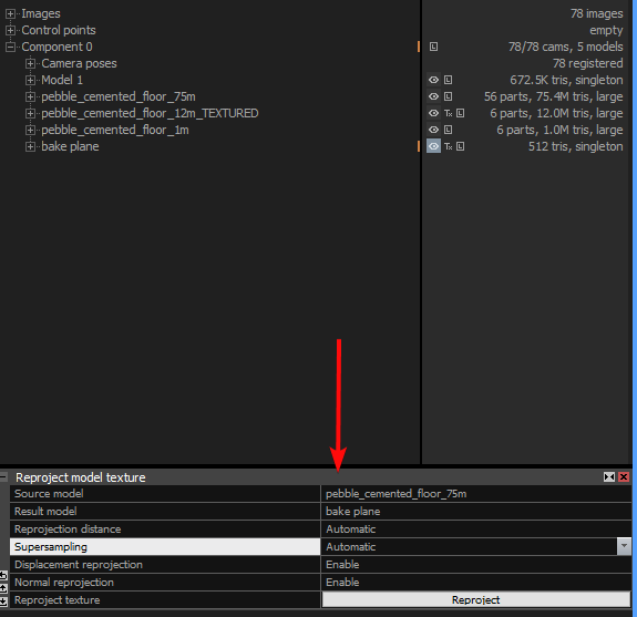
Make sure Reprojection Distance is set to Automatic (this can be changed to Custom if there are clipping errors with the bake), also set the Supersampling to Automatic. (Supersampling can be set to manual if we want somewhat smoother results. Generally either Automatic or 4x should be good, as anything above 4x will probably give diminishing returns at 8k resolution.)
And of course make sure Displacement reprojection and Normal Reprojection are both enabled.
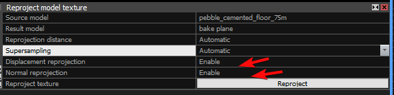
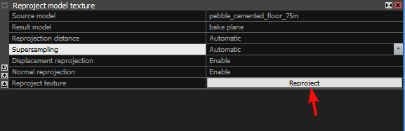
Click “Reproject”
- Once that’s done we can bake the color, we’ll change the Source model to the textured version, disable Normal and Displacement, enable Color reprojection, and make sure the source layer is set to 16-bit Color layer:
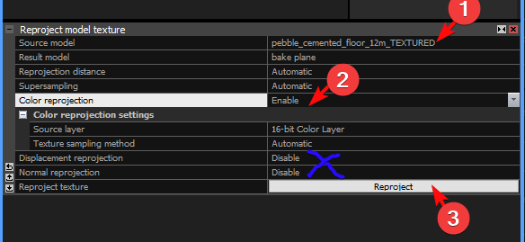
And then click Reproject again as shown above.
Exporting the baked textures from Reality Capture:
- Once our bakes are done we can export them as texture maps. We’ll select the bake plane, go to “Mesh Model” and click on “Dense Mesh Model” to export.
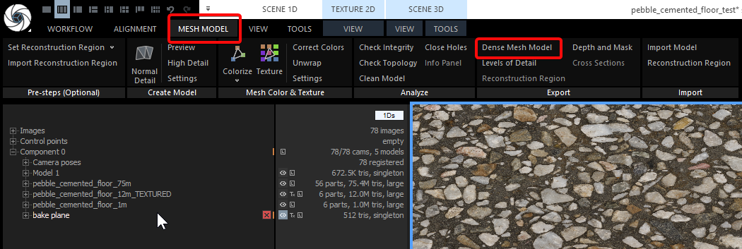
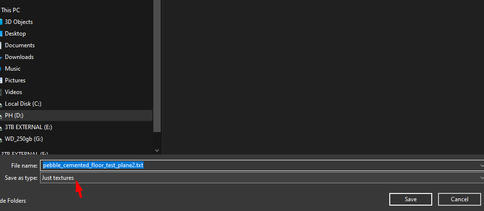
- We’ll set the type to “Just Textures” and click Save
Note: Reality Capture should not ask us for payment again, since of course we have already paid for this scan when we exported the proxy mesh earlier.
- In the export options, we’ll select the texture maps and formats we want to save out, then click OK. (preferably TIFF for the Normals and 16-bit Color, and EXR for the Displacement)
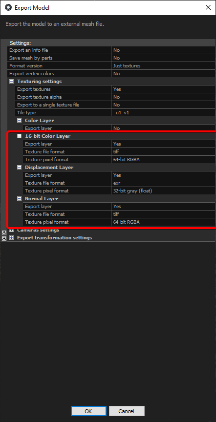
Note: the “Color Layer” in the above export window refers to the Vertex Colors, which we don’t need. The correct color channel here is the 16-bit Color Layer as shown.
- Now we just click “OK” and that’s it! We’ve saved out all our maps, and we can now continue to Unity ArtEngine to convert them into a seamless PBR texture set.
Step 5: Tiling in Unity ArtEngine
ArtEngine is a node-based application used for authoring high quality seamless PBR texture sets. It makes use of AI-based tools as well as conventional methods to modify and “mutate” existing textures. It has many different nodes and features that are useful on all kinds of material types, but we will only be looking at the basics in this guide.
NOTE: As of July 2022, ArtEngine is no longer actively maintained, but the standard version is still offered as a kind of perpetual free trial that works on Windows.Unity has stated that much of the functionality and AI-based tools will be available as part of their cloud-based toolset in the future.
To get started installing the free version, click here. (You will need a Unity ID account to use it)
Documentation and further help on getting started are available here
ArtEngine Interface Overview:
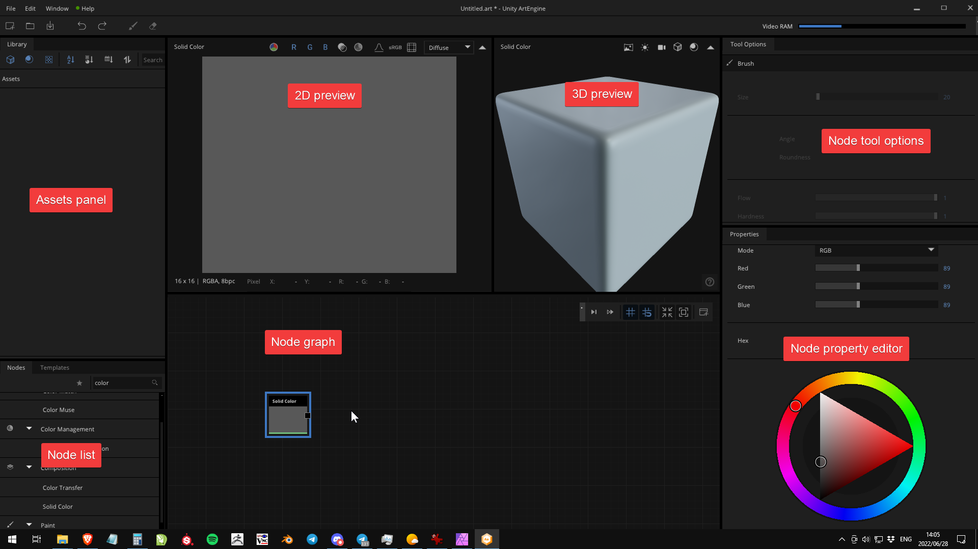
- Firstly we need to import our RealityCapture bakes into ArtEngine. Simply click and drag them into the node editor here:
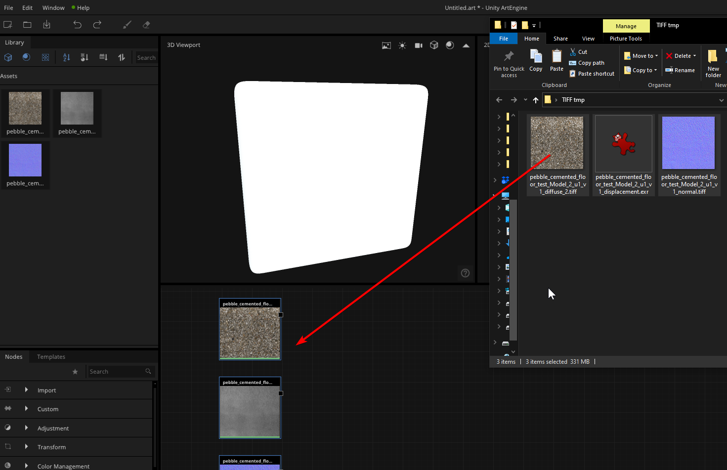
We now have 3 nodes in the Node Graph containing our baked map information. We can double click on a node to view it in the 2d/3d preview areas, and we can press TAB in the 2d view to get a tiling preview. (Use scroll to zoom and middle mouse to pan in the 2d, 3d and node-graph areas.)
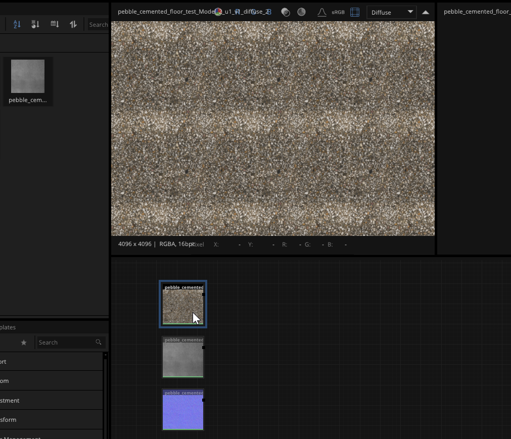
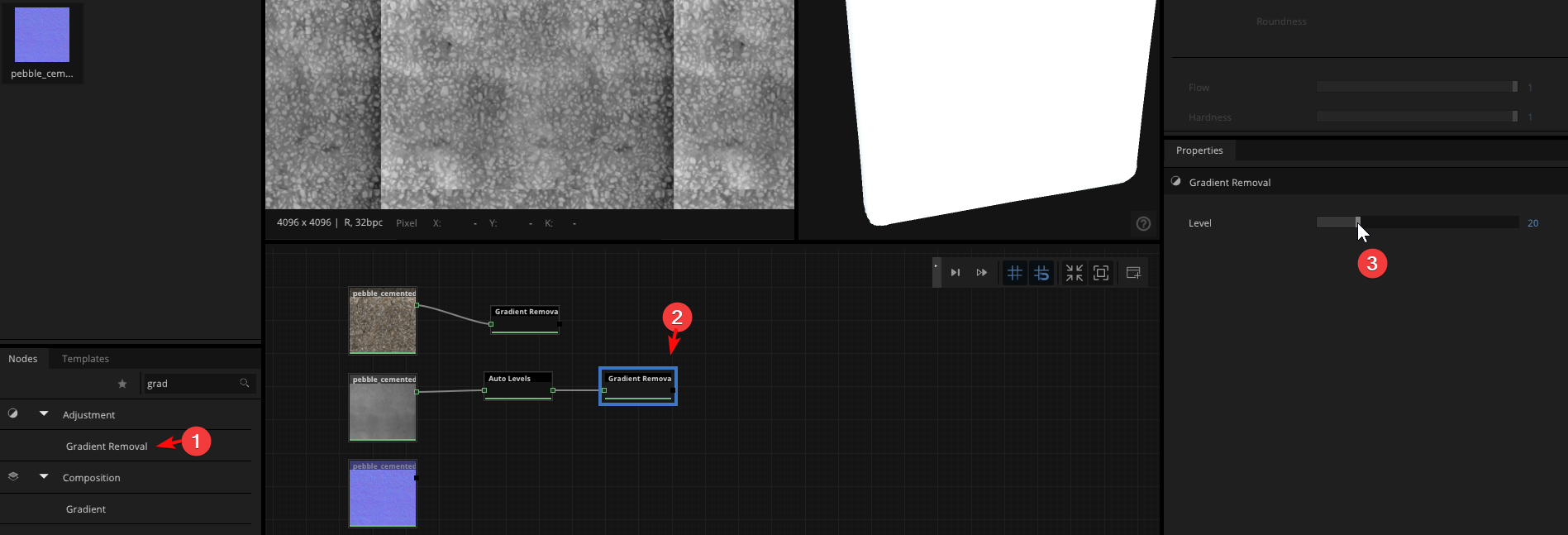
- We can see from the tiling preview on this particular map that it has a gradient, which is causing an obvious repetition when we zoom out. We can add a gradient removal node to help remedy this. In the Nodes panel on the left, search for Gradient Removal, and drag it into the node graph:
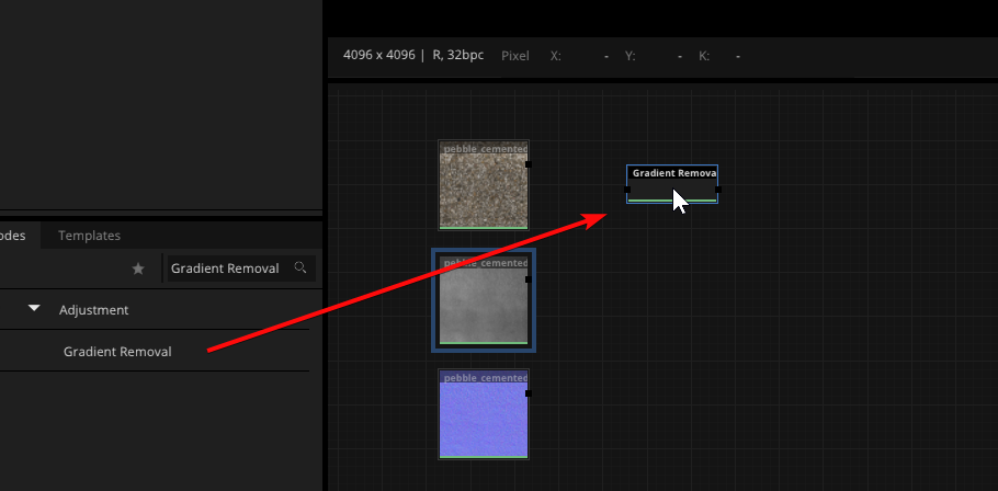
Now we can connect the color map to the gradient removal by dragging from the little square:
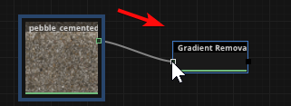
If we double-click on the gradient removal node, we can see it looks a lot better in the 2d preview. We can set the Gradient removal strength in the properties panel on the right. (Many nodes have extra settings here.)
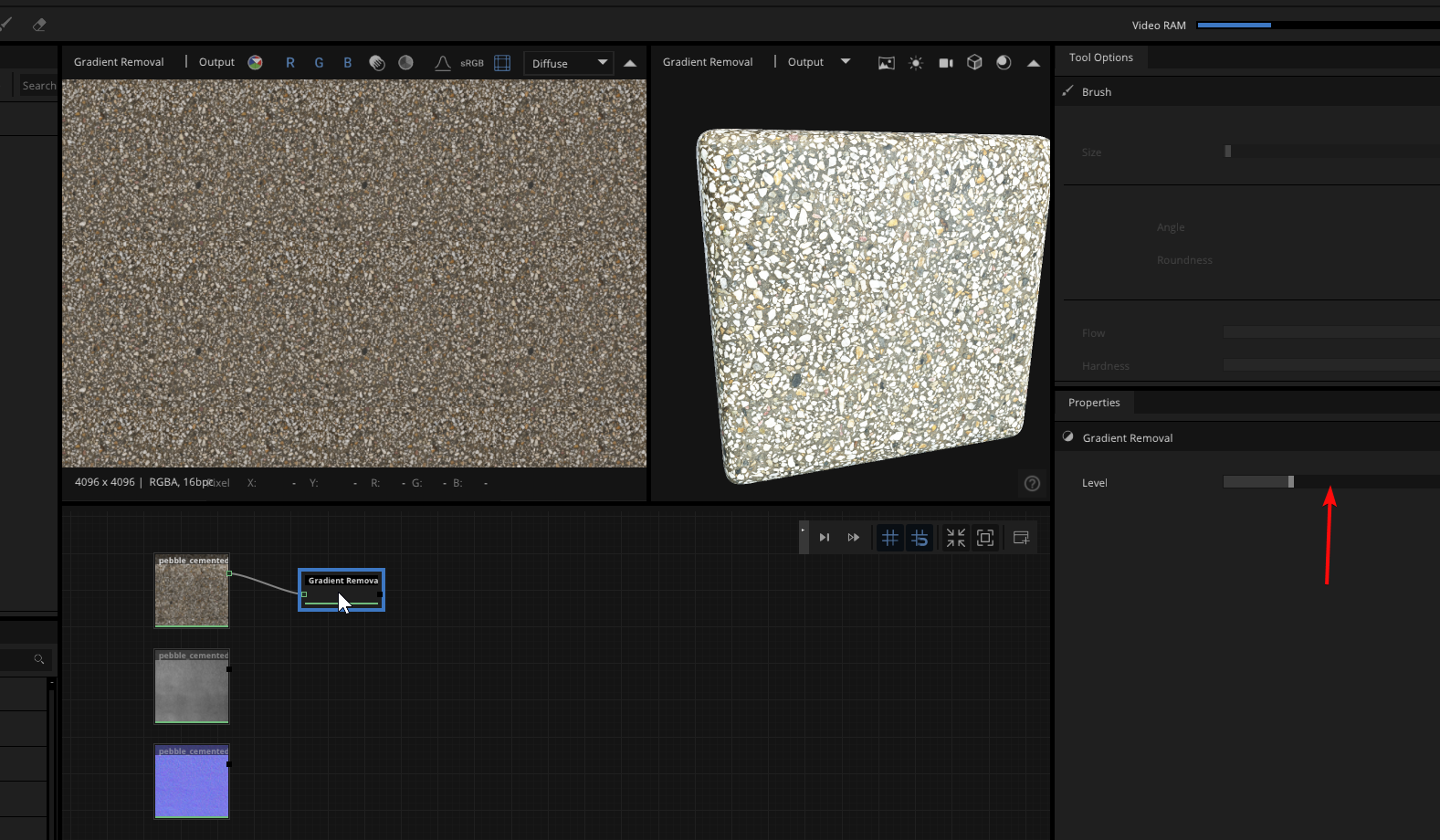
Note: It’s recommended to be as subtle as possible when working with effects like gradient removal. While useful, they can be pretty destructive, and may significantly change the original colors and values of our textures. Use the slider to find a good amount. Not too much or the texture will end up looking very bland and “CG”.
- We can double click the Displacement and normal maps to view their previews. The Normal map was saved from Reality Capture as a 16bit PNG, so it should show up fine, however the displacement map just shows black:
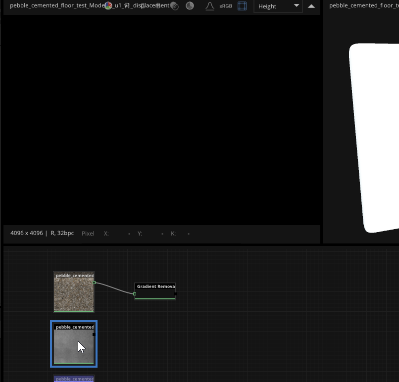
This is because it was saved as a 32bit EXR file. The displacement data is still there, but it’s showing black because the range is outside of what the image viewer or our screen can display. While it’s certainly possible to work with 32bit files in ArtEngine, it’s a bit overkill for us, and we’ll convert it to 16bit by putting it through an Auto-Levels node. This will also make it possible for us to preview it while working:
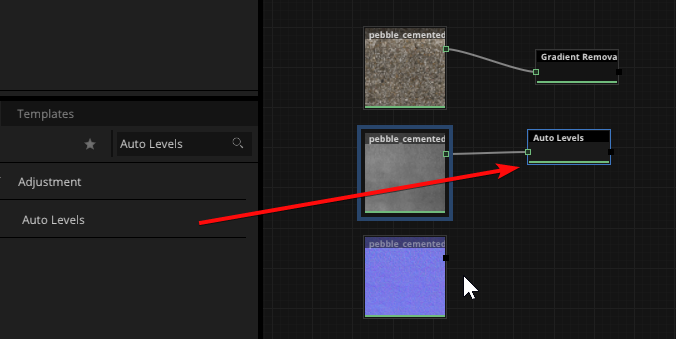
Now if we double-click on the Auto-levels node, we should see our Displacement map:
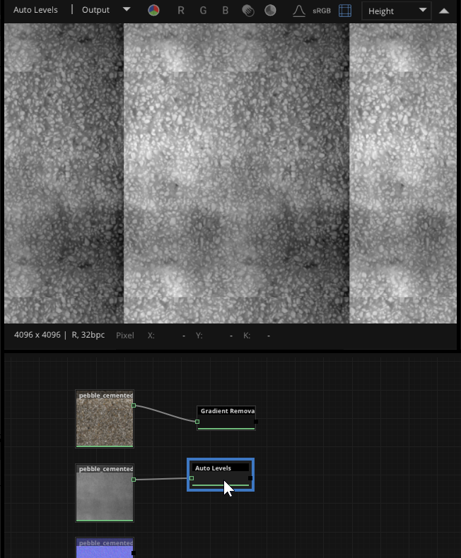
The Displacement also shows a pretty harsh gradient. We can reduce it the same way we did with the color map, by adding a Gradient removal node. Remember to keep this one subtle as well.
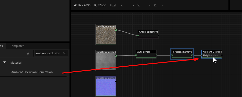
- We’ve adjusted the maps a bit, let’s go ahead and use the displacement information to generate an Ambient Occlusion map:
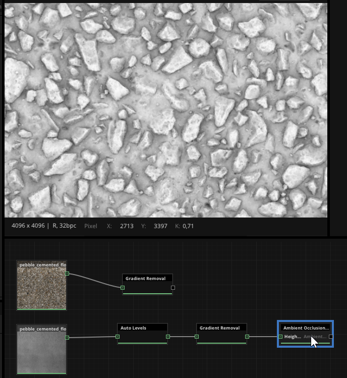
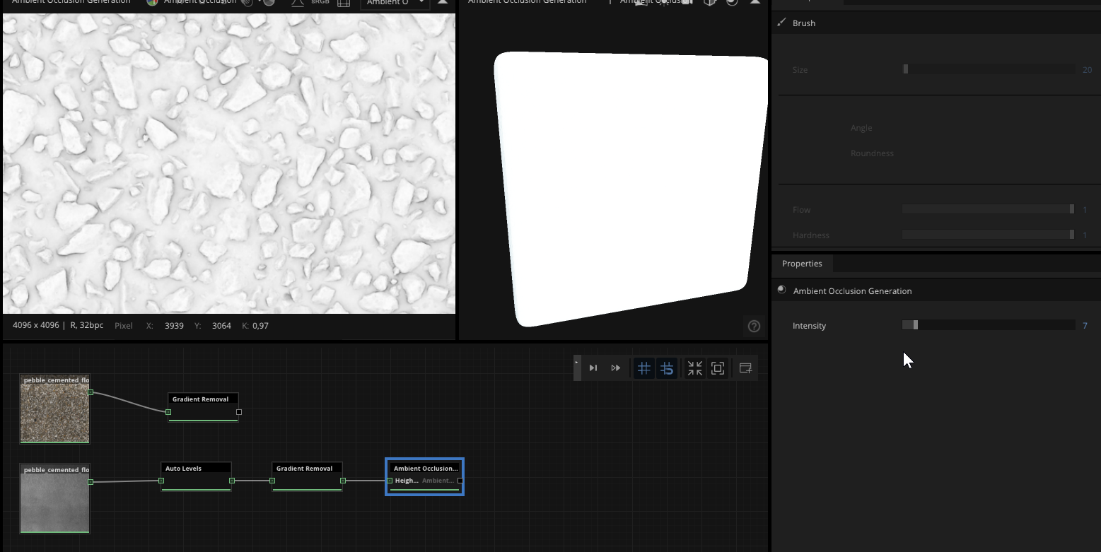
Double-click on the AO node to preview it:
We can see it’s pretty strong, for this kind of flat surface we don’t want it too harsh (this depends on the type of texture), let’s bring the strength down in the properties panel on the right:
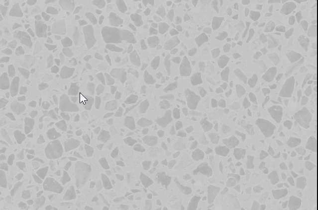
We can also generate a roughness map from the color information:
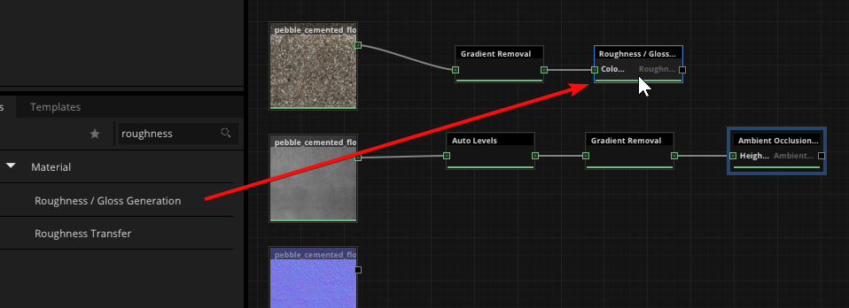
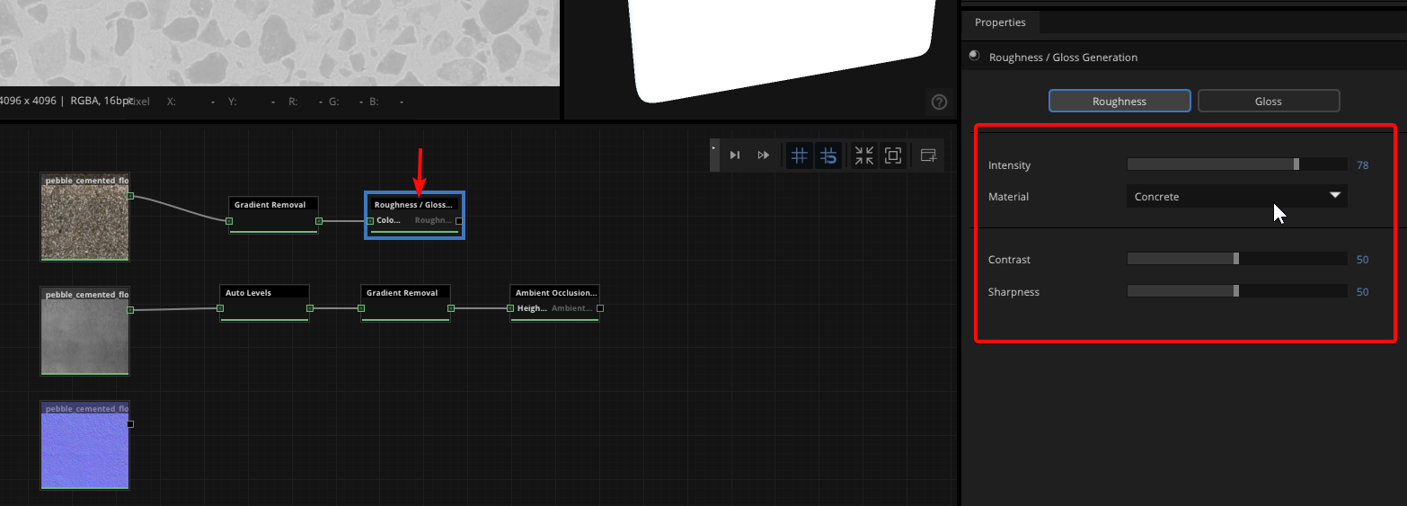
We know that this particular texture is not very smooth, so it will have a high roughness value overall. In PBR terms this means that the roughness map should be fairly bright, since a value of 1 (white) is 100% rough, while a value of 0 (black) is completely reflective/smooth. We’ll use the Concrete preset of the roughness node as a starting point, and if necessary use the intensity, contrast and sharpness sliders to tweak it further.
Note: Remember that in the real world no material is ever 100% shiny or 100% rough. While it’s possible to find some “official” roughness values for different materials online from various sources, in reality it’s often OK just to eyeball it, since even within particular material groups there will be a lot of variation depending on external factors. We can use the 3d preview to get an idea of how the roughness map behaves, or we can come back and tweak later after doing a proper render in Blender.
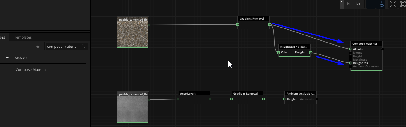
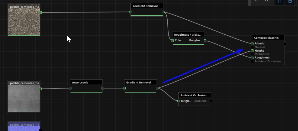
- Now that we’ve generated all the necessary maps, we can combine them into a material using the Compose Material node. We’ll route the information from the various stages in the node-chain to their appropriate slots. For example, the color gradient removal goes into the Albedo input, (“Albedo” is another term for “Color”) and of course Roughness goes to Roughness:
The displacement goes into “height”. Make sure to use the gradient-removed version:
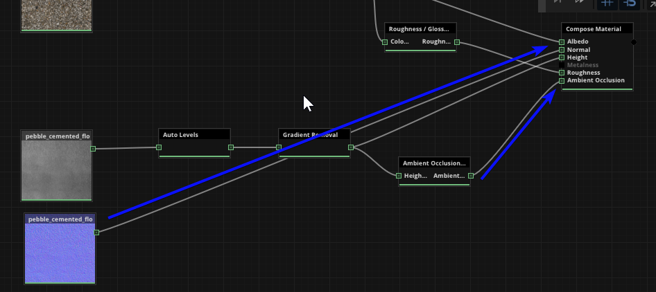
And the AO and Normal nodes are self explanatory:
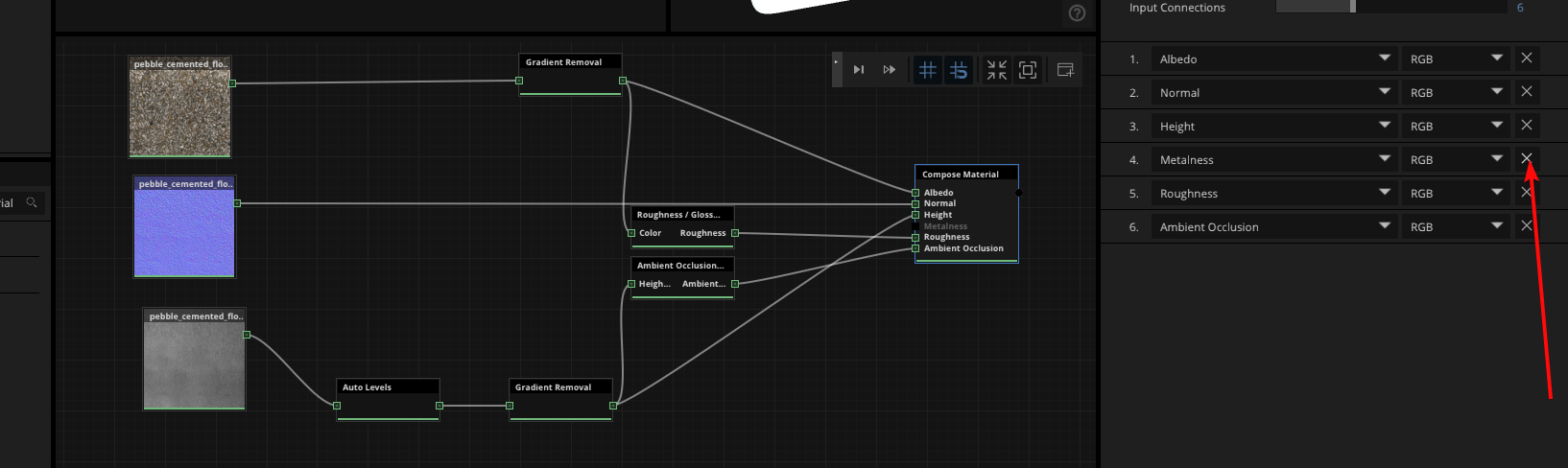
Now we have all the maps going to their correct inputs, notice we don’t have anything in the Metalness input, since of course this material contains no metallic information. We can remove the metalness input by clicking on the Compose Material node and clicking the X next to Metalness:
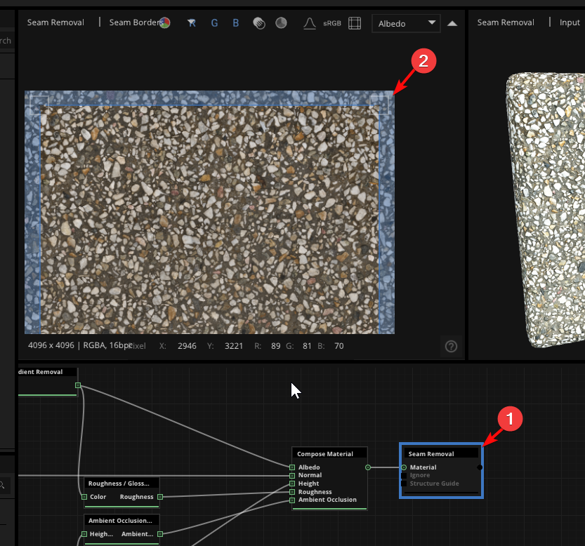
- We are now ready to add a Seam Removal node to the graph. (We only add the seam removal after the compose-material node, since we want to remove seams from all the maps at once)

If we double-click on the Seam Removal node we can see its preview in the 2d view. Here we can drag the blue box to define the area that will be affected during seam removal. We don’t want the blue area too narrow, since then the transition will be very obvious, but we also don’t want it too wide because then it affects too much of our texture. The default setting is usually close to correct on a random surface like this one.
Note: Different surface scans will need different treatment, and as a rule, random surfaces like the one shown here are easier to work with. Your approach might need to differ significantly if you’re working with a grid or brick pattern for example.
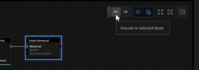
With the Seam Removal node selected, we can click the Execute button to start the seam removal process:
Once done, we can double click to preview it, and we can again hit TAB in the 2d view to toggle the tiling preview:
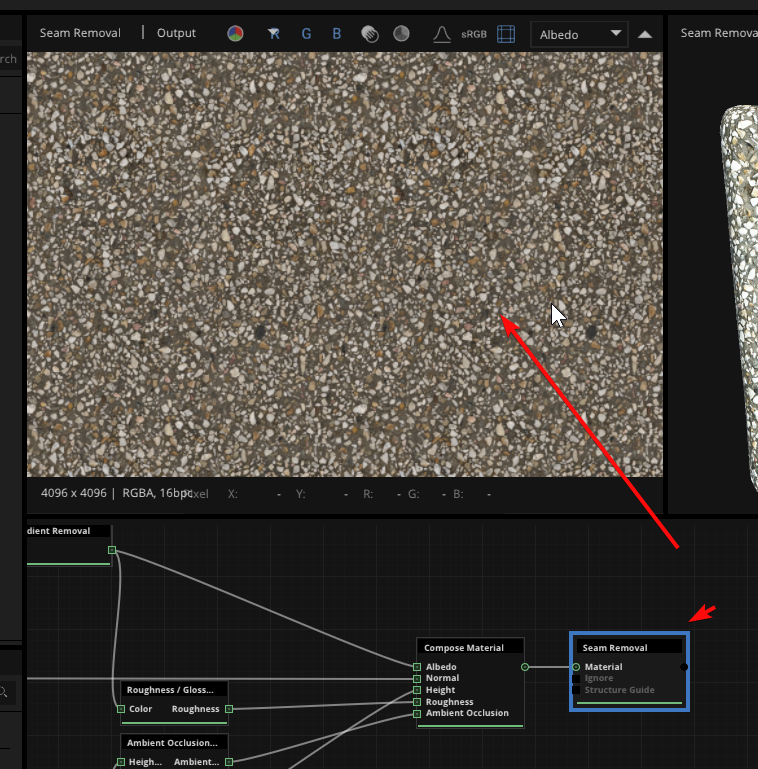
We can also preview the different maps in the material by clicking the little menu in the top right of the 2d view:
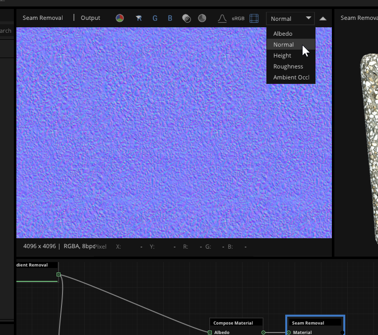
If done correctly, there should be no visible seams on any of the maps.
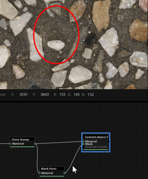
- The seam removal worked pretty well, but we can still adjust any areas that look a bit off. Let’s zoom in a bit and take a look at this slightly awkward fading shape here.
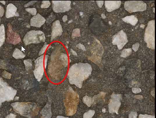
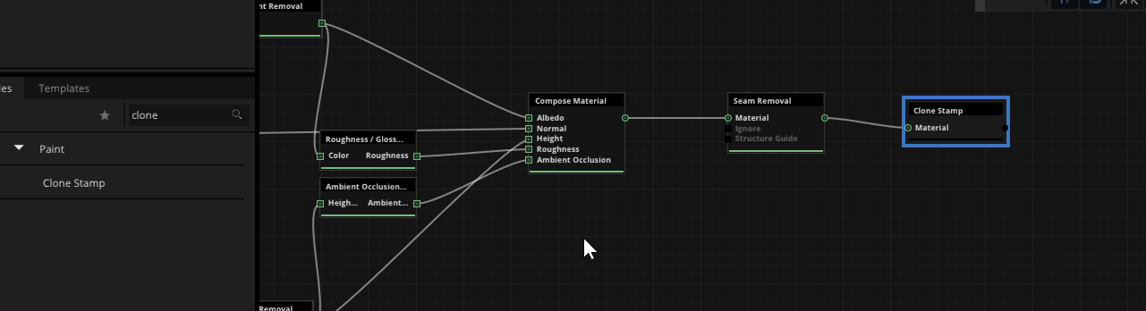
While there are several ways we can tackle this, for now we’ll go for a simple clone operation. Let’s connect a Clone Stamp node to our node-tree.
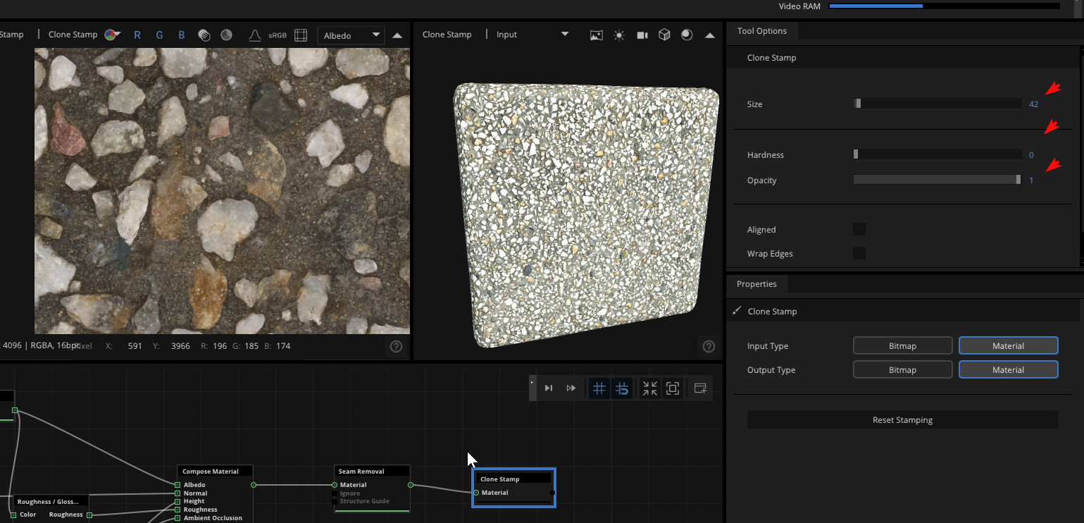
We’ll double-click on the clone stamp node to view its properties on the right, where we can set things like the size, hardness and opacity of our clone brush.
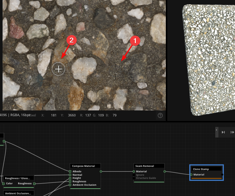
Once we’ve set our brush parameters, we can ALT+click in the 2d view to select a clone source, then just click and drag over any area to start cloning:
We’ll just copy some of the concrete over that awkward shape to hide it. We can ALT+click at any time to reset our clone source, and use CTRL+Z to undo any action.
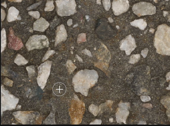
And so we can continue using the clone brush to fix any weird areas.
Note: The clone-stamp brush is just one of many methods at our disposal. We can also use nodes like the Content-Aware Fill node to fix up any areas that need work.

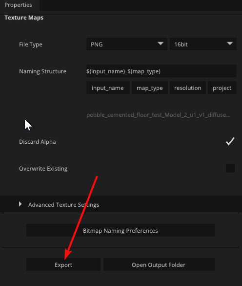
- Our maps are now ready to export. We can add an Output node and then set our export parameters on the right. It’s recommended to always use a 16 bit lossless format such as PNG.
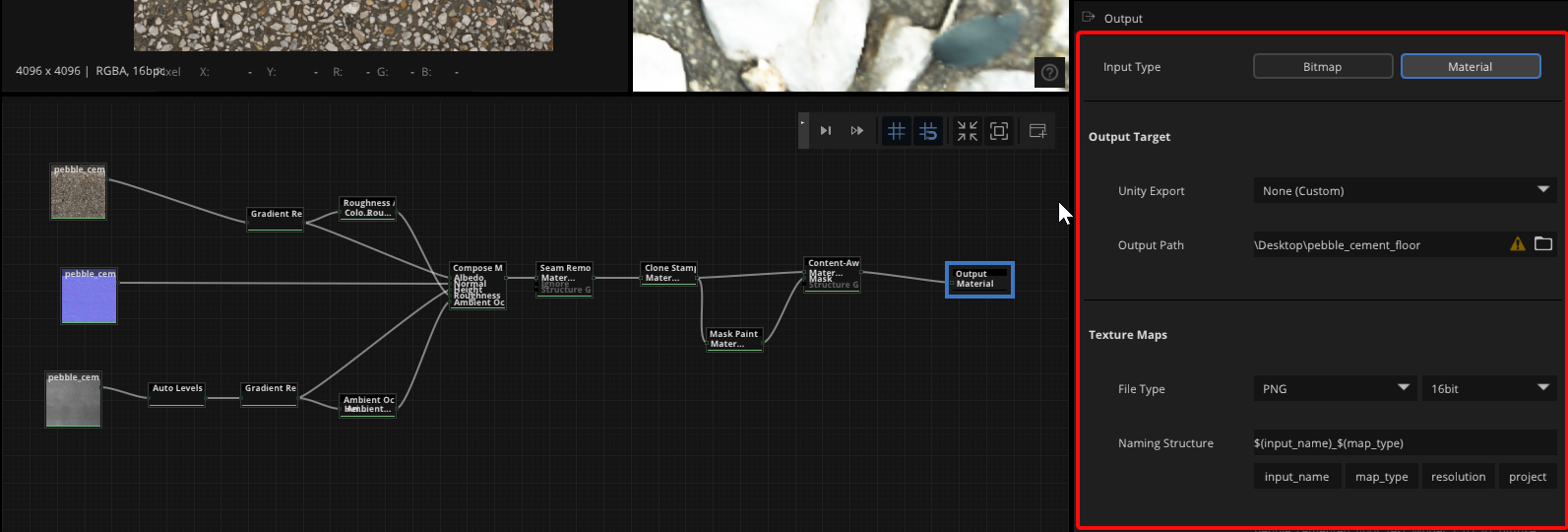
Now we can click Export at the bottom:
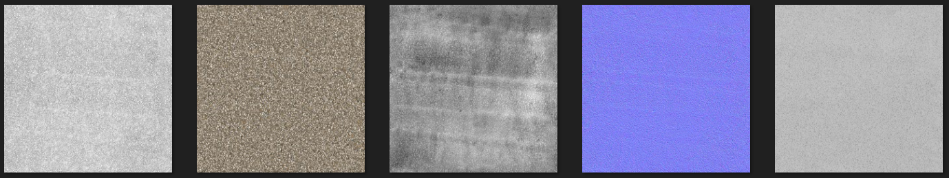
We finally have a fully tiling texture set! We were able to get a really nice result from just 3 maps and a relatively small node-tree.

Step 6: Material setup
Finally, we’re ready to assemble the texture maps into a material in Blender.We’ll set it up with Adaptive Subdivision for that nice crispy displacement detail.
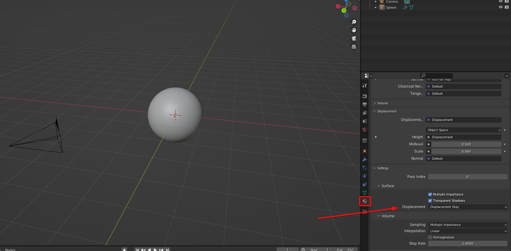
- First we’ll open Blender, delete the default cube and light, and add a Sphere. We’ll also add a material to the sphere and enable Displacement Only in the material settings.
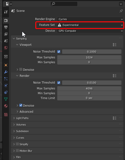
- We’ll enable the “Experimental” Feature Set in the render settings, and we can also enable GPU Compute if we have a Graphics card installed in our PC. (GPU rendering is generally much faster than CPU)
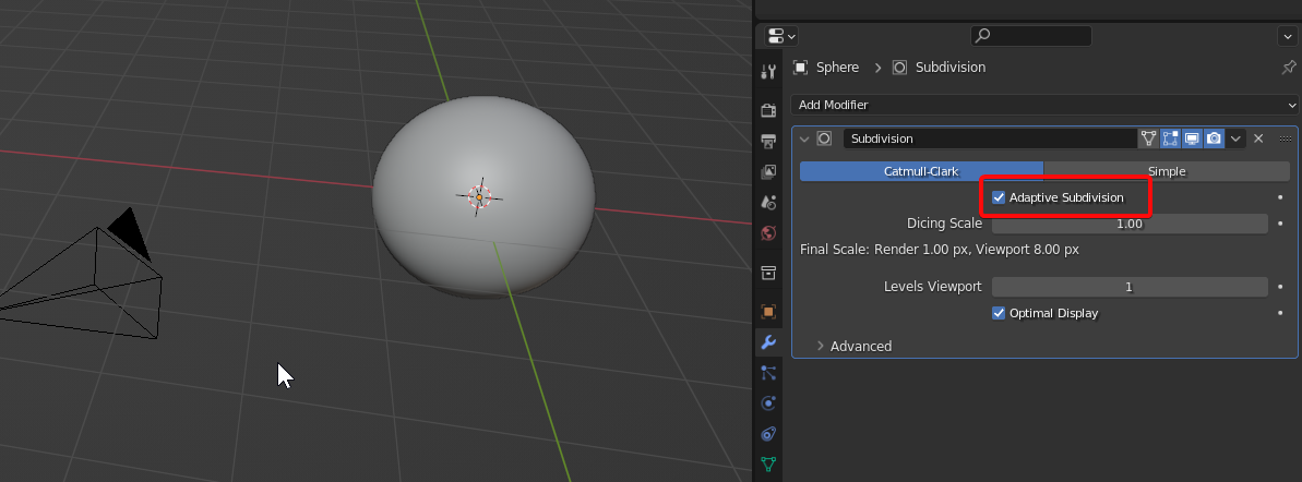
- We can add a Subdivision Surface modifier to the sphere, and enable Adaptive Subdivision (this only works if Experimental is turned on).
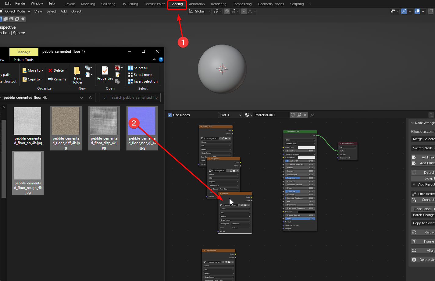
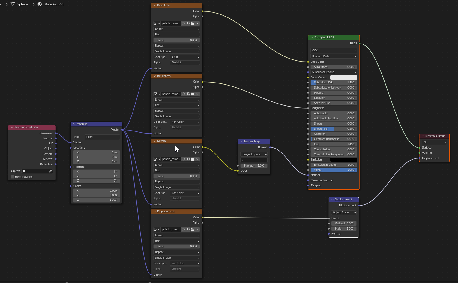
- Now we’ll go to the Shading tab and select our sphere to start setting up the material in the Node Editor. We can simply drag our texture maps into the node editor one by one. (We don’t need the AO map since it is only used in real-time engines like Eevee, or in game engines, or as a mask).
- We’ll connect our Diffuse (color) and Roughness maps to their respective sockets on the Principled BSDF node. Remember to set the Roughness map color space to non-color, since it’s an information map and doesn’t contain any color information.

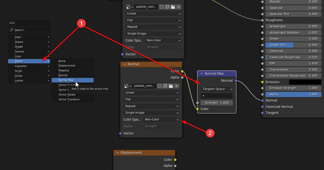
- We’ll need to press Shift+A and add a Vector > Normal Map node after the Normal texture map, and then connect it to the Normal socket on the main node. Again, remember to set the Color Space to Non-color or it will not render correctly.
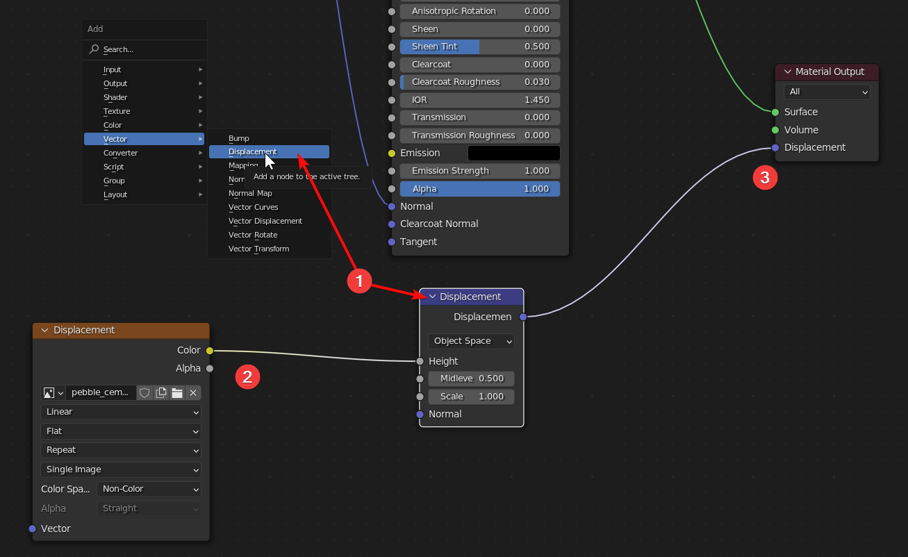
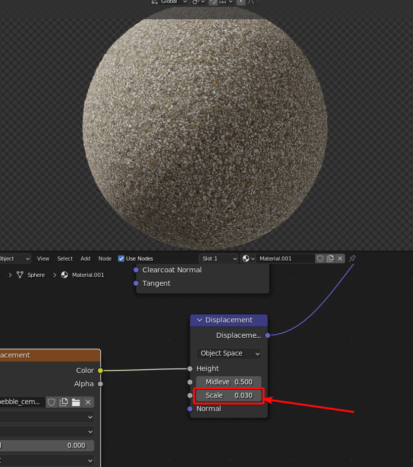
- Now We’ll hit Shift+A to add a Vector > Displacement node, and plug our Displacement map into its Height slot. Then plug the output into the Displacement socket on the Material Output. Remember to set the color space to non-color on the Displacement as well.
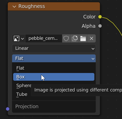
- Since we’re going to use generated texture coordinates for this preview, we’ll need to set the method on each texture map node from “flat” to “box”
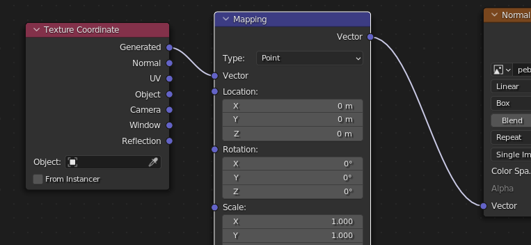
- Now we can hit Shift+A and add a Input > Texture Coordinate node and a Vector > Mapping node, and connect them to each input texture as shown below:
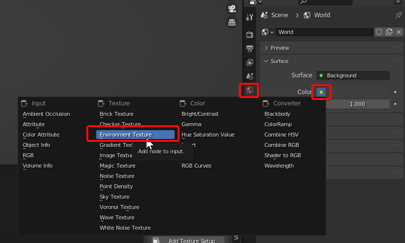
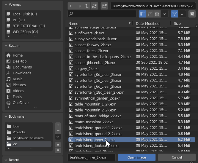
- Before we render we’ll also need to add a HDRI from for our lighting in the world properties (Lots of great free HDRIs available on polyhaven.com):
- We can try a test render by enabling viewport shading in the top right corner of the 3d view:
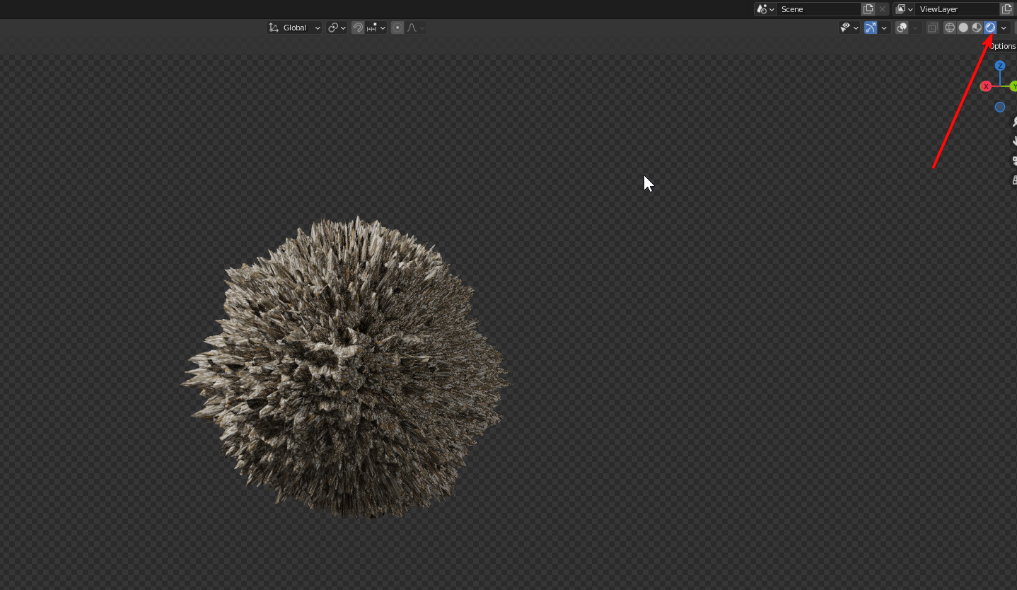
We see that our material is working, but it’s very spiky. This is because our displacement node is set way too strong. Let’s decrease it a bit by tweaking the scale value:
- Now we can do our final render by hitting F12 or by going to Render > Render Image
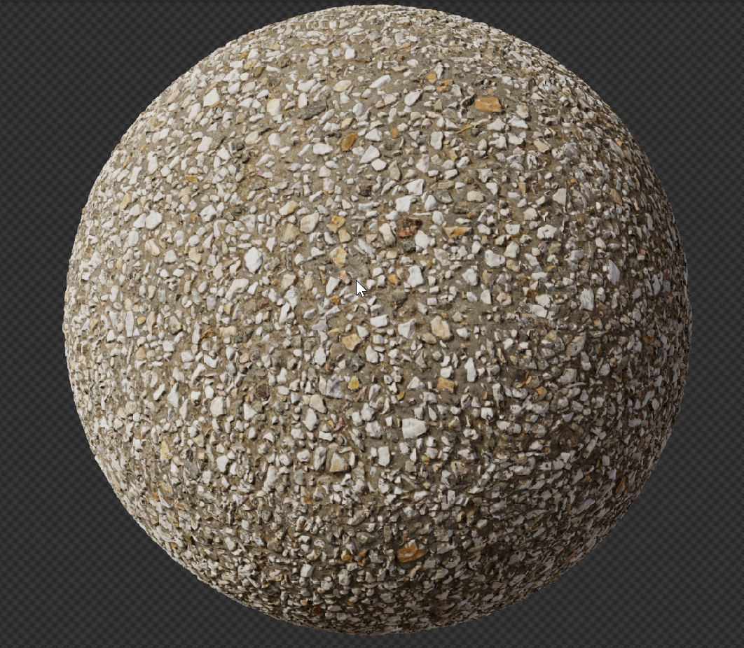
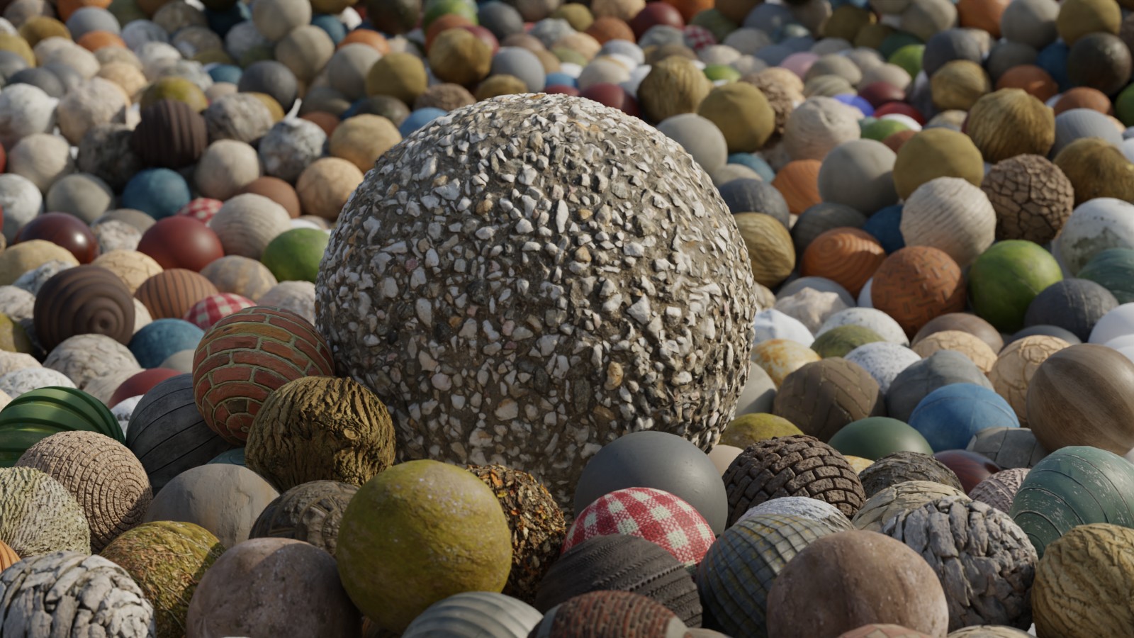
And we’re done! We’ve created a fully tiling photoscanned texture set.
Excelente, gracias!!!
This whole document really makes me appreciate the effort put into all the free stuff you have on here. tysm!
Thank you too!
How much time will approx take to create one material… through this process….??
While it depends, one could probably do it in 2-3 days. 1 day for shooting, and the remaining 2 days for cleanup/tiling etc. but it really depends on your level of experience and your camera, hardware, and so on. If you’re just starting out you should expect to spend quite a bit more time on the processing and tiling steps in particular.
Very informative and it makes me appreciate the high quality work you guys do! Thank you!
16 bit images in tiff format do not provide better textures. Furthermore, using 16 bit .tiff wouldn’t be wise either considering their lossless format is often larger than the original raws, for no realizable gain.
8 Bit jpeg’s suffice and RealityCapture only uses 8bit for mesh reconstruction, if it is fed 16 bit anything, it’ll convert them under the hood anyway to 8 bit.
The only time we ever need 16 bit anything in RC for texturing is on HDR images. There is no discernable quality difference between 16 bit and 8 bit. OR jpeg and tiff. Particularly in the realm of material scanning, where more often than not, the surface has no depth that would require HDR datasets.
We can’t import raws directly in Reality Capture as we need to correct for CA and other image artifacts first. Using a 16-bit format is ideal since 8-bit is not enough to contain the original raw data (which is typically 12 or 14 bits depending on the camera), particularly because we intend to do delighting on the texture later. 16-bit is indeed overkill for meshing, but we need the 16-bit for the texture to avoid introducing banding when doing delighting and color calibration from the chart.
PNG and EXR are other alternatives to TIFF, but in our test these are either slower or introduce other artifacts.
Way Cool! A very Informative article. Your content is very helpful for all designers.
Thanks.
glad you found it useful!
Great tutorial. Very detailed. Thankyou.
When creating textures of actual tiles, like you use on the floors/walls of houses, how do you photograph them?
I am using Blender for ArchViz shots of my new house to help us decide on the interior design details. In particular, choosing tiles for the kitchen and bathroom. Its no good using tile textures from say PolyHaven, because, while they look great, they are not the tiles we would actually be able to buy.
So, I go to our local tile shop, and we can bring home samples of tiles. Then I photograph them. But, we can generally only bring home one example of each tile. So when photographing them I dont get the variability that you would get in real life once you lay a whole floor or wall.
If you look at some tiles, they have variability, both in pattern and roughness. So, when you are preparing ‘proper’ textures of physical tiles like this, how do you guys actually do it?
Do you go out and buy a couple of square meters of tiles, lay them, grout them, then photograph it? Do you just get one tile, photograph it in a light box, and ‘tweak it for some variability?
Do you form a relationship with a tile vendor in order to get access to a whole box of each sort of tile?
Do you use photogrammetry and thus multiple photos of something small like a 200mm x 200m tile, to capture there roughness?
What’s the actual process you use? I can’t seem to find this information anywhere, and would really appreciate some advice.
thank you.
Hi Phill,
Thank you for the kind words.
To get our textures we often go out into the wild and find the surfaces.
Some of our materials have reference images to show some context as to where they were shot.
Check out this material as an example: https://polyhaven.com/a/park_sand
Currently we do not work with any vendors to get tiles though I do know that some Companies who specialize in Architectural renders for the purpose of showing customers what the finishing could look like do indeed speak to vendors and may have some arrangements.
In your situation I would recommend taking a look at a Substance Designer based workflow which would enable you to take one tile as reference and procedurally create patterns and variations of it with the ability of making it “Seamless” and tillable like our materials are.
I hope this helps.
Cheers!
– James
That is really awesome, thanks for sharing so helpful information.
Amazingly detailed post!
Thank you so much!
Im not sure where else to put this question but i feel its the most -on topic here. In your linked guide to shooting accurate base-color you say this: “In a nutshell, the white value we’re aiming for is [244, 244, 241] if you’re shooting in natural light, or [235, 232, 226] if you’re shooting with a cross-polarized flash (i.e. accounting for the lack of a specular component).”
Isn’t this wrong? If youre aiming for a basecolor of [244, 244, 241] the minimum 4% specular reflections will still get added on top if im not mistaken? the darkest patch is indeed around 50,50,50 rgb but when you render that in a PBR model, 4% specular will get added on top at f0 either way. resulting in a surface that’s too bright
Cross-polarized colors come out darker and more saturated because the specular component is not present. In this logic when shooting regularly without cross-polarization it would be a choice/trade-off between having an albedo thats slightly too bright and desaturated and an albedo that is roughly correct in it’s brightness (if you calibrate the non cross-polarized version to [235, 232, 226] anyway) but will just have slightly desaturated colors.
Its like choosing between having two things off or having one thing off?
I’d rather go for option 2!
Im trying to find a robust and “close enough” way of shooting srgb base color values for work and this is closest ive gotten. When I realized using color checker software with a color checker doesn’t result in a linear and accurate albedo, and in fact doesn’t correct the brightness at all. I almost punched my monitor.
Thanks so much for such a detailed Article. This is a great contribution to the CG Community . This is hands down the most well documented Article about Photoscan PBR creation I have seen online.
Hi there!
Since this article dates back to 2022, is the workflow still the same? I’m thinking in particular of ArtEngine, which is no longer updated. Have you found an alternative or are you still using it?
Very informative though, thank you.
This is a highly technical process.
No wonder there are so few textures / contributors.
And no wonder this stuff is so quality.